
Open-Source Internship opportunity by OpenGenus for programmers. Apply now.
In this article, we will be exploring a paper on “Adversarial examples in the Physical world” by Alexey Kurakin, Ian J. Goodfellow and Samy Bengio. This paper basically shows how machine learning models are vulnerable to adversarial examples.
In this paper has explored the concept of generating adversarial examples that are a threat to the machine learning models and comparison of different types o method is done. Some experimental analysis was also conducted where images were taken and accuracies were generated. These numerical results can be referred from the paper itself.
What is an Adversarial example?
An adversarial example is an item or input which is slightly modified but in such a way that it does not look different from the original example but the machine learning model misclassifies it. The modifications to the original examples are done in such a way that the user is unable to tell the difference but the model produces incorrect output.
Consider the image below:
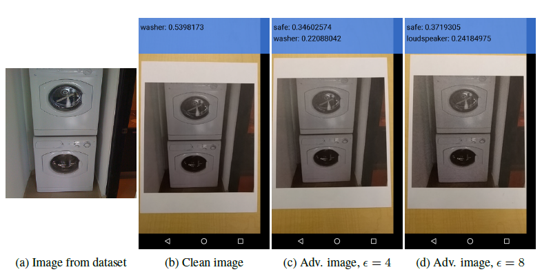
The image (b) is the clean image. Image (c) and (d) are adversarial images. Images (c) and (d) have adversarial perturbation 4 and 8 respectively.
Adversarial perturbation is basically a parameter or metric which shows how much the original image is changed.
Introduction
Now a days, models based on neural networks and other machine learning models are achieving great accuracies. In classification, there are so many great models that helps in getting the correct classification. But the important thing to point out is that these models are vulnerable to produce incorrect output when adversarial manipulations are done to the input. This problem can be summarized or represented in the following way:
Let M be a machine learning system and C be a clean input image. We will assume that the input C is correctly classified by the model i.e.
M(C)=Ytrue
It is possible to create an adversarial input A such that
M(A)!=Ytrue
Methods to generate Adversarial examples
Notations involved:
X- an image, typically a 3D tensor.
Ytrue- true class for the image X
J(X,y)- cross entropy cost function of the neural network.
Clip{}- function which performs per pixel clipping if image X' so the result will be in Linf neighbourhood of source image X.
- Fast Method: This is one of the simplest methods to generate adversarial example. In this method, the cost function is linearized and solving for the perturbation is done that maximizes the cost subject to Linf constraint. This may be done in closed form, for the cost of one call to back-propagation:
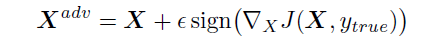
This method is called fast just because it is faster than other methods.
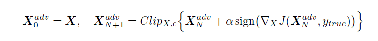
2. Basic iterative method: In this method, we apply the fast method multiple times with small step size and we will clip the pixel values of the intermediate results after each step to see that they are in sigma-neighborhood of the original image.
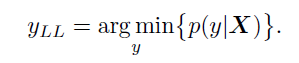
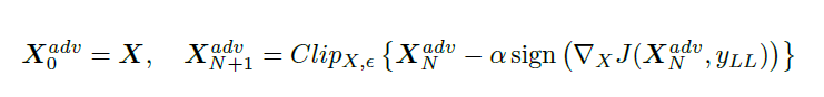
- Iteratively Least Likely Class method: In this method, the adversarial image will be produced which will be classified as a specific desired target class. For desired class we chose the least-likely class according to the prediction of the trained-on input image X.
For a well trained classifier, the class to which the image is misclassified is quite different from the real or correct class. For example the image of dog is classified as an airplane.
To make an adversarial image which is misclassified as yLL we maximize log p(yLL|X) by making iterative steps in the direction of sign{ deltaX log p(yLL|X). This last expression equals sign{-deltaX J(X,yLL)} for neural networks with cross entropy loss. Thus we have the following procedure:
Comparison of Methods of generating Adversarial examples
In this paper, experiments were done for comparison of the different methods for generating adversarial examples. Consider the following graphs:
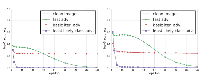
Now here we have the Top1 and Top5 classification accuracy against epsilon (adversarial perturbation) on clean and adversarial images. This was tested on the Inception v3 model and experiments were performed on 50,000 validation images from the ImageNet dataset.
What we observe from the results is that for Fast method, top1 accuracy decreases by a factor of 2 and top5 accuracy by about 40% even with smallest values of epsilon. Increasing the value of epsilon have not significant changes in the accuracy for this method until epsilon=32. After that accuracy begins to fall to almost 0 when epsilon=128.
For basic iterative method, it provides good adversarial images for epsilon<48 but after that there is no significant improvement.
The least likely class method even for small epsilon values produces images that will definitely be misclassified.
Destruction Rate
Destruction rate is basically a notation which is used to analyze the influence of arbitrary transformation in adversarial images. It can be defined as follows:
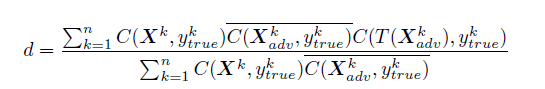
n- number of images used to compute destruction rate.
X^k- image from dataset
Ytrue^k- true class of X^k
Xadv^k- corresponding adversarial image
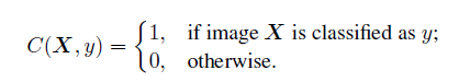
C(X,y)- indicator function which indicates whether image was classified correctly
Experimental observations on Image transformation
Based on the experiment conducted (refer paper for experiment details), the following observations were reported:
- Images generated by fast method are the most robust to transformations and the ones generated by iterative least likely are least robust.
- The top5 destruction rate is higher than top1 destruction rate.
- Changes in terms of brightness and contrast does not affect adversarial examples that much.
- Blur, noise and JPEG encoding have a higher destruction rate than changes in brightness and contrast.
Conclusion
So in this article, what we have learned is that no matter how much big dataset we train our machine learning model on, how much good accuracy we have achieved, there are possible adversarial examples with certain degree of changes with respect to the real example, that can be misclassified or in simple words, the machine learning model can be fooled.
For complete experiment analysis, the paper mention in the beginning can be referred as it contains specific experiment on the Inception v3 classifier.
Learn more:
- Explaining and Harnessing Adversarial examples by Ian Goodfellow by Murugesh Manthiramoorthi at OpenGenus
- Deep Neural Networks are Easily Fooled: High Confidence Predictions for Unrecognizable Images by Murugesh Manthiramoorthi at OpenGenus
- One Pixel Attack for Fooling Deep Neural Networks by Murugesh Manthiramoorthi at OpenGenus
- Machine Learning topics at OpenGenus