
Open-Source Internship opportunity by OpenGenus for programmers. Apply now.
Reading time: 30 minutes
Alexnet is a Deep Convolutional Neural Network (CNN) for image classification that won the ILSVRC-2012 competition and achieved a winning top-5 test error rate of 15.3%, compared to 26.2% achieved by the second-best entry.
Though there are many more network topologies that have emerged since with lot more layers, Alexnet in my opinion was the first to make a breakthrough.
Architecture:
Alexnet has 8 layers. The first 5 are convolutional and the last 3 are fully connected layers. In between we also have some ‘layers’ called pooling and activation.
The network diagram is taken from the original paper.
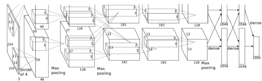
The above diagram is the sequence of layers in Alexnet. You can see that the problem set is divided into 2 parts, half executing on GPU 1 & another half on GPU 2. The communication overhead is kept low and this helps to achieve good performance overall.
Layer 1
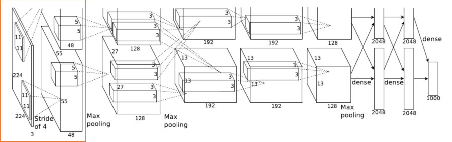
- Layer 1 is a Convolution Layer,
- Input Image size is – 224 x 224 x 3
- Number of filters – 96
- Filter size – 11 x 11 x 3
- Stride – 4
- Layer 1 Output
- 224/4 x 224/4 x 96 = 55 x 55 x 96 (because of stride 4)
- Split across 2 GPUs – So 55 x 55 x 48 for each GPU
You might have heard that there are multiple ways to perform a convolution – it could be a direct convolution – on similar lines to what we’ve known in the image processing world, a convolution that uses GEMM(General Matrix Multiply) or FFT(Fast Fourier Transform), and other fancy algorithms like Winograd etc.
I will only elaborate a bit about the GEMM based one, because that’s the one I have heard about a lot. And since GEMM has been, and continues to be, beaten to death for the last cycle of performance, one should definitely try to reap it’s benefits.
Benifits
- Local regions in the input image are stretched out into columns.
- Operation is commonly called im2col.
- E.g., if the input is [227x227x3] and it is to be convolved with 11x11x3 filters with stride 4
- Take [11x11x3] blocks of pixels in the input
- Stretch each block into a column vector of size 11113 = 363.
- Result Matrix M = [363 x 3025] (55*55=3025), 55 comes from 227/4
- Weight Matrix W = [96 x 363]
- Perform Matrix multiply: W x M
Disadvantages of this approach:
- Needs reshaping after GEMM
- Duplication of data – due to overlapping blocks of pixels, lot more memory required.
Layer 2
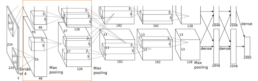
- Layer 2 is a Max Pooling Followed by Convolution
- Input – 55 x 55 x 96
- Max pooling – 55/2 x 55/2 x 96 = 27 x 27 x 96
- Number of filters – 256
- Filter size – 5 x 5 x 48
- Layer 2 Output
- 27 x 27 x 256
- Split across 2 GPUs – So 27 x 27 x 128 for each GPU
Pooling is a sub-sampling in a 2×2 window(usually). Max pooling is max of the 4 values in 2×2 window. The intuition behind pooling is that it reduces computation & controls overfitting.
**Layers 3, 4 & 5 follow on similar lines.
Layer 6
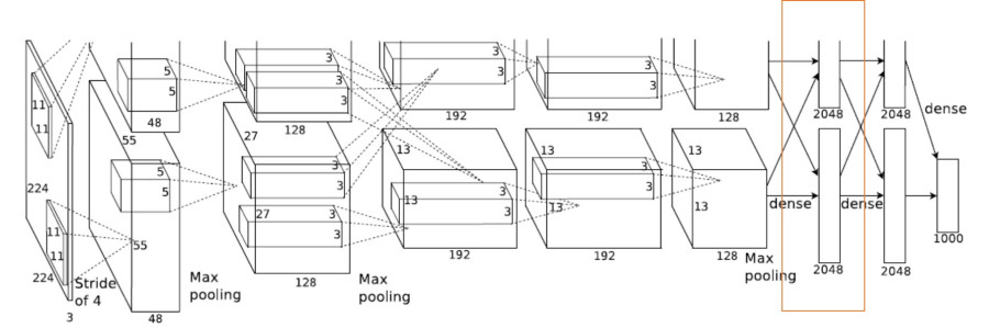
- Layer 6 is fully connected
- Input – 13 x 13 x 128 – > is transformed into a vector
- And multiplied with a matrix of the following dim – (13 x 13 x 128) x 2048
- GEMV(General Matrix Vector Multiply) is used here:
Vector X = 1 x (13x13x128)
Matrix A = (13x13x128) x 2048 – This is an external input to the network
Output is – 1 x 2048
**Layers 7 & 8 follow on similar lines.
Uses:
The results of AlexNet show that a large, deep convolutional neural network is capable of achieving record-breaking results on a highly challenging dataset using purely supervised learning. Year after the publication of AlexNet was published, all the entries in ImageNet competition use the Convolutional Neural Network for the classification task. AlexNet was the pioneer in CNN and open the whole new research era. AlexNet implementation is very easy after the releasing of so many deep learning libraries.
[PyTorch] [TensorFlow] [Keras]
Comparison with latest CNN models like ResNet and GoogleNet
AlexNet (2012)
In ILSVRC 2012, AlexNet significantly outperformed all the prior competitors and won the challenge by reducing the top-5 error from 26% to 15.3%. The second place top-5 error rate, which was not a CNN variation, was around 26.2%.
GoogleNet(2014)
The winner of the ILSVRC 2014 competition was GoogleNet from Google. It achieved a top-5 error rate of 6.67%! This was very close to human level performance which the organisers of the challenge were now forced to evaluate. As it turns out, this was actually rather hard to do and required some human training in order to beat GoogLeNets accuracy.
ResNet(2015)
At last, at the ILSVRC 2015, the so-called Residual Neural Network (ResNet) by Kaiming, introduced a novel architecture with “skip connections” and features heavy batch normalization. Such skip connections are also known as gated units or gated recurrent units and have a strong similarity to recent successful elements applied in RNNs. Thanks to this technique they were able to train a NN with 152 layers while still having lower complexity than VGGNet. It achieves a top-5 error rate of 3.57% which beats human-level performance on this dataset.