In a previous post on CART Algorithm, we saw what decision trees (aka Classification and Regression Trees, or CARTs) are. We explored a classification problem and solved it using the CART algorithm while also learning about information theory.

In this post, we show the popular C4.5 algorithm on the same classification problem and look into advanced techniques to improve our trees: such as random forests and pruning.

C4.5 Algorithm for Classification

The classification problem discussed in the previous post was regarding Loan Application Approval. Here is a quick recap of the problem:

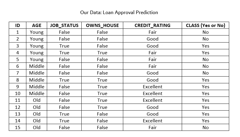
Our example problem is a binary classification problem. Each record is for one loan applicant at a famous bank. The attributes being considered are - age, job status, do they own a house or not, and their credit rating. In the real world, banks would look into many more attributes. They may even classify individuals on the basis of risk - high, medium and low.

Here is our data:

And here is the goal:
Use the model to classify future loan applications into one of these classes:
 Yes (approved) and  No (not approved)

Let us clasify the following applicant whose record looks like this:
Age: Young
Job_Status: False
Owns_House: False
Credit_Rating: Good

The metric (or heuristic) used in C4.5 to measure impurity is the Gain Ratio. We select the attributes with higher Gain Ratio values first. Gain Ratio favors smaller partitions with many distinct values, which is different from the splitting criterion used in the CART algorithm (the Gini Index).

Formally, C4.5 is a recursive greedy algorithm that uses Divide-and-Conquer. Here is the algorithm:

//C4.5 Algorithm
INPUT: Dataset D
1. Tree = {}
2. if D is "pure" or stopping criteria are met
    3.then terminate
4. for all attributes A in D
    5.compute information criteria if we split on A
6. A_best = best attribute calculated above
7. Tree = {A_best} (tree has A_best in the root node)
8. D' = sub-datasets of D based on the root node
9. for all D' do
    10. Tree' = C4.5(D')
    11. Join Tree' to the corresponding branch in Tree
12. return Tree 
OUTPUT: Optimal Decision Tree 

Solving this Example Problem

We need to first define Entropy, which is used to find the Information Gain, and ultimately the Gain Ratio that will be used to select the best attribute as a root node. Entropy is the degree of randomness (or, uncertainity) and for our processed information is calculated as:

Entropy = -∑p(I)*log₂p(I)

We first find the global entropy of the entire dataset D:
Entropy(D) = -6/15.log₂(6/15) - 9/15.log₂(9/15) = 0.971
[As there are 6 No and 9 Yes values for the 15 total records]

Information gained by selecting attribute A to branch/partition the data is called Gain(A) and is calculated for each attribute A_i:

•  Gain(A) = Entropy(D) - Entropy(A, D)
  

So we first calculate Entropy(A_i, D) for each attribute A. This is the expected entropy if A_i is used as the current root of the tree:

Entropy(A_i, D) = ∑ |D_j|/|D| x Entropy(D_j)

This becomes clear when we apply it for our problem:

Entropy(Owns_House) = (6/15).Entropy(D₁) + (9/15).Entropy(D₂)
= (6/15)x0 + (9/15)x0.918
=0.551
[D1 is the subset of records with No, and D2 is the subset of records with Yes]
Gain(Owns_House) = 0.971 - 0.551 = 0.420

Similarly,
Entropy(Age) = (5/15).Entropy(D₁) + (5/15).Entropy(D₂) + (5/15).Entropy(D₃)
= 0.888
[D1, D2, D3 are sub-datasets for Young, Middle and Old]
Gain(Age) = 0.971 - 0.888 = 0.083

Entropy(Job_Status) = (5/15).Entropy(D₁) + (10/15).Entropy(D₂)
= 0.647
Gain(Job_Status) = 0.971 - 0.647 = 0.324
[D1, D2 are sub-datasets for True and False]

And,
Entropy(Credit_Rating) = (4/15).Entropy(D₁) + (5/15).Entropy(D₂) + (6/15).Entropy(D₂)
= 0.608
[D1, D2, D3 are sub-datasets for Fair, Excellent and Good]
Gain(Credit_Rating) = 0.971 - 0.608 = 0.363

Finally, we need to calculate gain ratios for each attribute. This is a step that used to be skipped in ID3.
The formulae required for Gain Ratios are given below:

• GainRatio(A) = Gain(A) / SplitInfo(A)
  

• SplitInfo(A) = -∑ |Dj|/|D| x log2|Dj|/|D
  

We choose the attribute with the highest gain to branch/split the current tree.

We shall show how to calculate the Gain Ratio for Owns_House. The same steps are followed for the other attributes, but they will all have gain ratios that are lower.


SplitInfo(Owns_House) = -6/15.log₂(6/15) - 9/15.log₂(9/15) = 0.971
[As there are 6 Yes and 9 No values for Owns_House being True or False.]
Finally,
GainRatio(Owns_House) = 0.420/0.971 = 0.432
Exercise - find the gain ratios for other attributes and check if they are lower!

ID3 -

The older ID3 algorithm is the same except that the step of calculating Gain Ratios is skipped. The metric that is used is Information Gain. Incidently, the attributes all have lower information gains than Owns_House as well, and so the optimal decision tree will be the same here: but this method does not work all the time and is the reason why ID3 had to be upgraded to C4.5.

This higher Gain Ratio is why Owns_House will be chosen as the root node. This entire process will repeat (until the stopping criteria are met) to determine the next best node and then the next - till we have the best possible decision tree. We can lookup the tree to then classify future records.

This is how we ultimately arrive at this decision tree (which is the same as obtained using CART in the previous post!)-

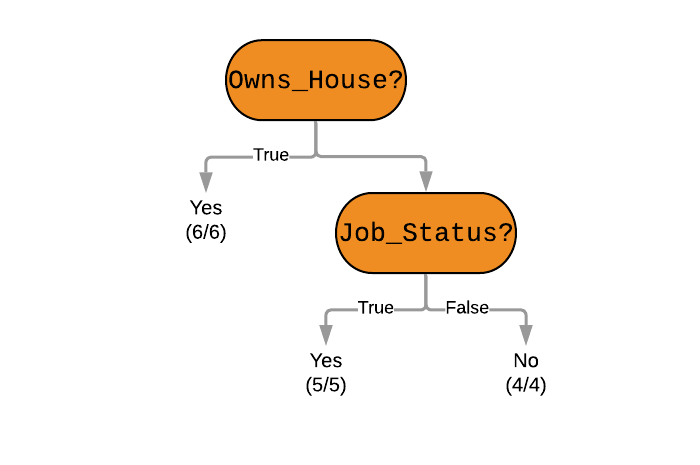
We can see that the in our problem the applicant does not own a house, and does not have a job. Unfortunately, his loan will not be approved.

Advanced Methods To Improve Performance

Pruning

Pruning is a fancy English word for trimming a tree. We can prune our decision tree to make them shorter and simpler - which is something we desire, as shown in the previous post.

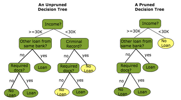
The idea is to remove sections of the tree that provide little power to classify instances (less information gain). This shall reduce the complexity of the final classifier, and hence improves the predictive accuracy (by reducing the chances of overfitting).

Pruning can occur in a top-down or bottom-up approach. A top-down approach traverses des and trims subtrees (starting from the root), while a bottom-up approach starts at the leaf nodes. Below is a simple pruning technique:

Reduced Error Pruning
1. Start at the leaf nodes
2. Replace each node with its most popular class
3. Keep this change if prediction accuracy does not go down
4. Repeat for all leaf nodes

This is a naive, but simple and speedy approach.

Something more complex would be cost complexity pruning (also called weakest link pruning) where a learning parameter is used to check whether nodes can be removed based on the size of the sub-tree.

Random Forests

While pruning is an effective way to prevent over-fitting, Random Forests are a newer and cooler way to do so. This is a mini-dive into the world of Ensemble Learning techniques. These techniques essentially have a simple idea: improve your predictive performance by combining multiple ML algorithms together. But they get very complicated very quickly.

You may have heard of the word ensemble together - a very French word that means "together". In movies, an ensemble cast is a large cast full of some big name actors. Movies such as the Avengers series or the LoTR trilogy had ensemble casts. Even movies such as the Oscar-winning Spotlight(2015) featured an ensemble cast.

How do we create an ensemble cast of machine learning models?

Bagging

Bagging can be used to create an ensemble of trees where multiple training sets are generated with replacement. Bagging is a cool way to say "bootstrap aggregating", which is the actual name of this method.

Given a training set X = x1, ..., xn with responses Y = y1, ..., yn, bagging repeatedly (B times) selects a random sample with replacement of the training set and fits trees to these samples. This is where the "random" part in the name "random forests" comes from.

//Bagging
For b = 1, ..., B:
Sample, with replacement, n training examples from X, Y; call these Xb, Yb.
Train a classification or regression tree fb on Xb, Yb.

After training, predictions for new records x' can be made by averaging the predictions from all the individual regression trees on x'. In the case of classification trees, this is done by taking the majority vote, as shown below:

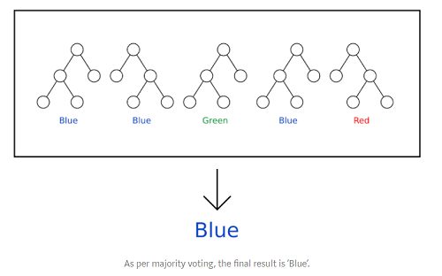
Here is some intuition to why such an ensemble approach would work: it is called the Wisdom of Crowds. If you have seen game shows like KBC (Who Wants to Be a Millionaire), contestants sometimes resort to polling the live audience to find the right answer. They trust the wisdom of the crowd -

“A large number of relatively uncorrelated models operating as a committee will outperform any of the individual constituent models.”

In our case, these models are decision trees.

Random forest ensures that each individual tree is not too correlated with the behavior of any other tree in the ensemble model by using random feature selection and bagging.

References

Test Yourself