
Open-Source Internship opportunity by OpenGenus for programmers. Apply now.
Elastic Net Regularization is a regularization technique that uses both L1 and L2 regularizations to produce most optimized output. This is one of the best regularization technique as it takes the best parts of other techniques.
We have started with the basics of Regression, types like L1 and L2 regularization and then, dive directly into Elastic Net Regularization.
What is Regression ?
Regression is a statistical method of estimating the relationship between a dependent variable and series of other variables and using this relation to predict the dependent variables on the basis of given variables.
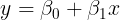
In Linear Regression we assume the estimating relation to be linear. Let's assume a simple example consisting only two variables, let y be the dependent variable and x be the other variable or feature as called in statistical terms.
Therefore let our estimated line be :
We have to calculate β0 and β1 in such a way that we fit our data best i.e. we must make sure that the difference between the estimated value and the actual value remains as minimum as possible.
There are many different methods of measuring error, but the one best suited is Ordinary Least Squares(OLS).
OLS is a function of β0 and β1 which is stated as follows :
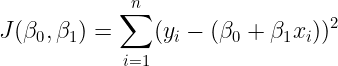
We have to minimize the above function, therefore the above function is referred to as the cost function
Thus by using calculus we can find out β0 and β1 using Gradient Descent.
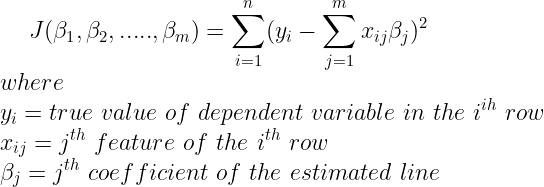
The same concept is applicable to a bigger dataset of n dimensions, in that case our parameters will be β0,β1......βn.
This is a brief summary of Linear Regression. For more detailed explanation you can refer below article on OpenGenus
Meaning of Coefficients
Regression models are the machine learning models which are fairly easy to understand and therefore easy to interpret. What do I mean by interpretation. Let's consider the example used above. Have you ever thought what does β0 and β1 signify ? β1 is the change in y for a unit change in x when all other features are held constant(In this case there is only one feature so, it doesn't matter but when we have more than one features we have to keep others constant). Similarly, β0 is the amount of y when x is 0. In case of only one features it looks easy, right ? Have you ever thought what happens when we have more than one feature and they are correlated among themselves ?
Why Regularization ?
Vanilla Linear Regression works fine in most of the cases but in cases where the features or independent variables are strongly correlated among themselves causes an increase in error. To picture this let’s say we’re doing a study that looks at a response variable — patient weight, and our predictor variables would be height, sex, and diet. The problem here is that height and sex are also correlated and can inflate the standard error of their coefficients. Thus there is a need for a better method which considers this aspect also.
Mathematical Notations
Since in practical scenarios we mostly have more than one features, therefore we must slightly change our mathematical notations. Let n is the number of rows in our dataset and m is the number of columns in our dataset.
Therefore our new cost function will be :
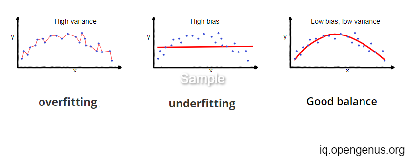
A look at Variance and Bias!
Variance is the measure of how spread our data is. In Linear Regression, the more is the variance the better we fit our training data, but it causes overfitting as our model fails to correctly predict test data. Bias is the distance between the true value and average prediction. We can think of bias as the degree to which we approximate our line. Thus, increasing bias agains harms our accuracy as error increases. There is a tradeoff between variance and bias and we have to adjust accordingly to increase accuracy
At best we come up with a model which minimizes both bias and variance(which doesn't happen usually!).
Ridge and Lasso Regression
We have seen that we underestimate the error that we get from our estimated output and the true value. Thus there is a need to add some penalty to our cost function. There are two ways in which we can penalize the cost function these are L1 Regularization and L2 Regularization.
We know that cost function is

L1 Regularization
In L1 Regularization we add the absolute value of coefficients as a bias.
A regression model that uses L1 regularization technique is called Lasso Regression
Cost function of Lasso Regression
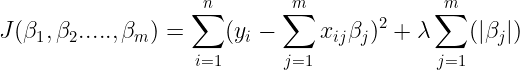
If lambda is zero then we will get back OLS whereas very large value will make coefficients zero hence it will under-fit.
L2 Regularization
L2 Regularization adds “squared magnitude” of coefficient as penalty term to the cost function
A regression model that uses L1 regularization technique is called Ridge Regression
Cost function of Ridge Regression
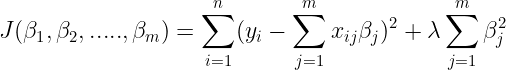
Here, if lambda is zero then you can imagine we get back OLS. However, if lambda is very large then it will add too much weight and it will lead to under-fitting. Having said that it’s important how lambda is chosen. This technique works very well to avoid over-fitting issue.
Elastic Net Regularization
The third type of regularization,(you may have guessed by now) uses both L1 and L2 regularizations to produce most optimized output.
In addition to setting and choosing a lambda value elastic net also allows us to tune the alpha parameter where 𝞪 = 0 corresponds to ridge and 𝞪 = 1 to lasso. Simply put, if you plug in 0 for alpha, the penalty function reduces to the L1 (ridge) term and if we set alpha to 1 we get the L2 (lasso) term.
Cost function of Elastic Net Regularization
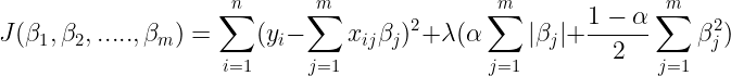
Therefore we can choose an alpha value between 0 and 1 to optimize the elastic net(here we can adjust the weightage of each regularization,thus giving the name elastic). Effectively this will shrink some coefficients and set some to 0 for sparse selection.
Example in Python
Let's take a random regression sample from scikit-learn's built in random dataset and train our model
    import numpy as np
    import pandas as pd
    import matplotlib.pyplot as plt
    import seaborn as sns
    from sklearn.linear_model import ElasticNet
    from sklearn.datasets import make_regression
    from sklearn.model_selection import train_test_split
    from sklearn import metrics
    X, Y = make_regression(n_features=4, random_state=0)
    data = pd.DataFrame(data = X,columns="F1 F2 F3 F4".split())
    data["Ouput"] = Y
    data.head()
    X_train,X_test,Y_train,Y_test = train_test_split(X,Y,test_size = 0.35)
    model = ElasticNet(alpha = 0.25)
    model.fit(X_train,Y_train)
    predictions = model.predict(X_test)
    print('MAE:', metrics.mean_absolute_error(Y_test, predictions))
    print('MSE:', metrics.mean_squared_error(Y_test, predictions))
    print('RMSE:', np.sqrt(metrics.mean_squared_error(Y_test, predictions)))
Some insights of the predicted results:
MAE: 10.106154003186473
MSE: 162.00975398346705
RMSE: 12.728305228248852
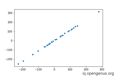
The above figure resembles a straight line which implies that our preditions are mostly correct
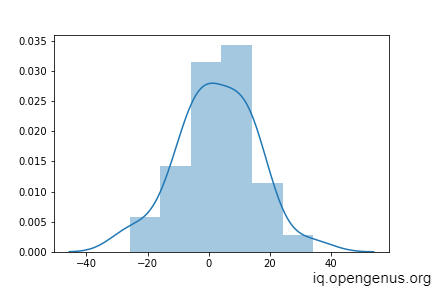
The distribution of the difference of Y_true and predictions is approximately normal with mean close to 0 which implies that most of the predicted values are almost close to the true value but there are some exceptions as well.
Conclusion
In this article we revised the basic math behind the linear regression model and explored the limitations and flaws of these models. We also explored the differenct type of corrections taken so far to improve model performance. We saw how we reached the concept of Elastic Net Regularization.
Check out exciting machine learning algorithms on OpenGenus here