
Open-Source Internship opportunity by OpenGenus for programmers. Apply now.
Reading time: 35 minutes | Coding time: 10 minutes
In this post, I will try to explain to you one of the most popular deep learning techniques known as Transfer Learning. We will see what exactly it is, why it works along with a Python implementation for the image recognition tasks.
What is Transfer Learning?
As per the recent advancements in technology, it has become relatively very easy to collect more and more data, which in turn requires a higher computation time for training a deep learning model. It can simply take from some hours to days to weeks months or even more :).
So, should we sit idle and stare at our laptop screens and wait for our model to get trained? NO ;) This is where the transfer learning comes to the rescue.
The most self-explained and straightforward definition of transfer learning can be referred to A process where a model trained on one problem is used in some way on a second related problem. Generally, an existing neural network model is trained on a large dataset on a problem similar to the problem that is being solved. One or more layers from this existing pre-trained model are then used in the new model trained on the problem of interest.
In the transfer learning technique, a model is trained on some huge standard dataset, which is later used for some other problem, which can be both similar or not so similar. In simple words, the pre-trained model uses its learned features on different sets of problems by transferring its knowledge. Thus the training time is reduced, and in turn, good results are achieved.
To achieve decent accuracy, it is always good to have a large dataset. But while working on a particular task, it is not always possible to have a massive quality dataset. Thus, it is always desired to have some benchmark datasets and models which already have outperformed numerous different existing models, so that we can use them as a feature extractor or for initialization purposes for our model of interest.
One famous example in the image recognition task is the ImageNet dataset, which contains around 1.2 million images with 1000 different categories. Some popular pre-trained models on this dataset are VGG16, Inception-V3, ResNet-50 etc..
Why Transfer Learning?
Transfer learning has become a new trend in the community of Deep Learning. It can be summarized due to these reasons-
-
In practice a very few people train a ConvNet from scratch (random initialization) since it is difficult to obtain an enough sized dataset. Infact, even after using data augmentation strategies, it is difficult to achieve a decent accuracy.
-
Due to insufficient sized dataset or million of parameters, overfitting becomes a significant reason for impacting the model's performance.
-
Using pre-trained network weights as initializations or a fixed feature extractor solves most of the problems.
-
Since neural networks can become extremely deep, it becomes extremely computationally expensive to train them even with high end computing power machines.
-
Determining the hyperparameters for a deep learning model is also not a cup of tea.
In a nutshell, these Deep Learning networks learn and try to detect edges in the earlier layers, Shapes in the middle layer, and some high-level data specific features in the later layers. These trained networks are generally helpful in solving several computer vision problems.
Transfer learning scenarios
There exists 4 different cases if we observe a relationship between new and original dataset. As we know, CNN features are somewhat general in the starting/early layers and as we go deep down in the network more specific and complex features are learned. The four possible situations can be explained using this diagram:
| CASE | TARGET DATASET | BASE TRAINING DATASET |
|---|---|---|
| CASE 1 | SMALL | SIMILAR |
| CASE 2 | LARGE | SIMILAR |
| CASE 3 | SMALL | DIFFERENT |
| CASE 4 | LARGE | DIFFERENT |
Possible Approach for each case
Case 1-
- Overfitting possible if trained from scratch.
- Remove original FC layer at end of pre-trained CNN model and add custom FC layer with required target classes.
- Randomize weights of new FC layer + freeze all weights from pre-trained model + train network to update weights of new FC layer.
Case 2-
- Overfitting not a major concern.
- Remove original FC layer at end of pre-trained CNN model and add custom FC layer with required target classes.
- Randomize weights of new FC layer + unfreeze all weights from pre-trained model(initialize other layers weight using pre-trained model) + retrain whole network to update weights.
Case 3-
- Overfitting possible if trained from scratch.
- Utilize low-level features(more specific) from pretrained model.
- Remove initial layers of pretrained model and use layers in the end of network using appropriate FC layer + freeze weights of pre-trained model -> Train to update weights of new FC layers.
Case 4-
- Train CNN from scratch
A neural network is generally trained on huge amount of data and gains knowledge from the data, which is compiled as weights of the network. The weights of a neural network can be extracted and then transferred to a other neural network.
Now, instead of training the other neural network from scratch, we transfer the learned features, which is the beauty of transfer learning. This is how existing weights are used, which in the implementation part simply refers to using the pre-trained model for the required task.
One analogy to identify why transfer learning works so well is that if a person knows how to make tea, then he definitely knows how to boil the water.
Implementation
We will see transfer learning technique for Dogs vs Cats classification. Link-
You can create a new kernel on Kaggle and execute following code to achieve a decent accuracy using VGG16.
Importing necessary packages:
import numpy as np
import pandas as pd
import matplotlib.pyplot as plt

from keras import layers
from keras import models
from keras import optimizers
from keras.preprocessing.image import load_img, img_to_array, ImageDataGenerator
from keras import applications

from sklearn.preprocessing import LabelEncoder
from sklearn.model_selection import train_test_split
from sklearn.linear_model import LogisticRegression
from sklearn import metrics
from sklearn.model_selection import cross_val_score

import glob
import os
Assiging path to data and image dimensions for VGG16 model.
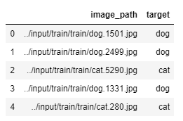
A dataframe with each image path and required target(cat or dog) is created.
IMAGE_FOLDER_PATH="../input/train/train"
FILE_NAMES=os.listdir(IMAGE_FOLDER_PATH)
WIDTH=150
HEIGHT=150

targets=list()
full_paths=list()
for file_name in FILE_NAMES:
    target=file_name.split(".")[0]
    full_path=os.path.join(IMAGE_FOLDER_PATH, file_name)
    full_paths.append(full_path)
    targets.append(target)

dataset=pd.DataFrame()
dataset['image_path']=full_paths
dataset['target']=targets

dataset.head(5)
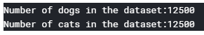
Printing target counts of both cats and dogs.
target_counts=dataset['target'].value_counts()
print("Number of dogs in the dataset:{}".format(target_counts['dog']))
print("Number of cats in the dataset:{}".format(target_counts['cat']))
Here, we're using the pre-trained VGG16 model
model used- VGG16
imagenet means download weights of VGG16 model trained on ImageNet dataset
include_top=False implies fully-connected output layers of the model used to make predictions is not loaded-> allows a new output layer to be added and trained
model=applications.VGG16(weights="imagenet", include_top=False, input_shape=(WIDTH, HEIGHT, 3))
model.summary()
Loading the data in batches (since 25,000 images) and showing progress after every 2500 images.
counter=0
features=list()
for path, target in zip(full_paths, targets):
    img=load_img(path, target_size=(WIDTH, HEIGHT))
    img=img_to_array(img)
    img=np.expand_dims(img, axis=0)
    feature=model.predict(img)
    features.append(feature)
    counter+=1
    if counter%2500==0:
        print("[INFO]:{} images loaded".format(counter))
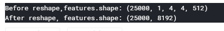
Reshaping the feature vector
features=np.array(features)
print("Before reshape,features.shape:",features.shape)
features=features.reshape(features.shape[0], 4*4*512)
print("After reshape, features.shape:",features.shape)
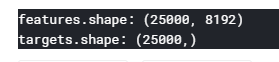
Label encoding the targets
le=LabelEncoder()
targets=le.fit_transform(targets)
print("features.shape:",features.shape)
print("targets.shape:",targets.shape)
Splitting the dataset into train and test
X_train, X_test, y_train, y_test=train_test_split(features, targets, test_size=0.2, random_state=42)
Training a simple logistic regression on extracted features
clf=LogisticRegression(solver="lbfgs")
print("{} training...".format(clf.__class__.__name__))
clf.fit(X_train, y_train)
y_pred=clf.predict(X_test)
Printing the results
print("Accuracy:",metrics.accuracy_score(y_test, y_pred))
print("Confusion Matrix:\n",metrics.confusion_matrix(y_test, y_pred))
print("Classification Report:\n",metrics.classification_report(y_test, y_pred, target_names=["cat", "dog"]))
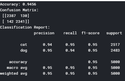
Conclusion
In this post, we saw how using simple series of steps we applied transfer learning technique and achieved a decent accuracy within few minutes. There exists a large number of pre-trained models,do make sure to check them out and also apply then to the same problem like ResNet50, Inception-V3, AlexNet etc. Not only for the problem of image recognition but also problems like in the domain of NLP can be solved using transfer learning like using pre-trained model like BERT.
Happy Transfer Learning :)