Image to Image Translation using CycleGANs with Keras implementation

Reading time: 40 minutes

Image to image translation is a class of computer vision and graphics, & deep learning problems where the goal is to learn the mapping between an input image and an output image using a training set of aligned image pairs.

Obviously, for most tasks, paired training data won't be available because:

1. Obtaining paired training data can be difficult and expensive
2. Acquiring input-output pairs for graphic tasks like artistic stylization can be even more difficult as the desired output is highly complex, often requiring artistic authoring and guidance.
3. For many problems, such as object transfiguration (e.g. generating an image of a horse from a given image of a zebra), the desired output is not even well-defined.

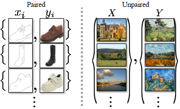
In the image above, paired training data (left) consists of training examples ${\left\{x_i, y_i\right\}}_{i = 1}^N$ where the correspondence between $x_i$ and $y_i$ exists.

Unpaired training data (right), consists of a source set ${\left\{x_i\right\}}_{i = 1}^N \left(x_i \in X\right)$ and a target set ${\left\{y_j\right\}}_{j = 1} \left(y_j \in Y\right)$, with no information provided as to which $x_i$ matches which $y_j$.

A need for an algorithm was felt which could learn to translate between domains without using paired input-output examples.

In their innovative paper titled, "Unpaired Image-to-Image Translation using Cycle-Consistent Adversarial Networks", Isola et al. (2018) achieve just this.

They presented an approach for learning to translate an image from a source domain $X$ to a target domain $Y$ in the absence of paired examples.

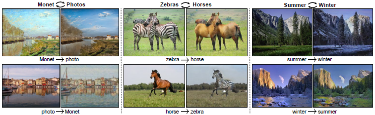
The above image illustrates the basic idea of the algorithm - Given any $2$ unordered image collections $X$ and $Y$ , the algorithm learns to automatically "translate" an image from one into the other and vice versa.

They assumed that there is some underlying relationship between the domains - for example, that they are $2$ different renderings of the same underlying scenery - and sought to learn that relationship.

Though they lacked supervision in the form of paired examples, they exploited supervision at the set-level:
Given one set of images in domain $X$ and a different set in domain $Y$, the authors trained a mapping $G: X \to Y$ such that the output $\stackrel{\wedge }{y} = G\left(x\right), x \in X$ is indistinguishable from images $y \in Y$ by an adversary which is trained to classify $\stackrel{\wedge }{y}$ from $y$.

The objective of their algorithm was to learn a mapping $G: X \to Y$ such that the distribution of images from $G\left(X\right)$ is indistinguishable from the distribution $Y$ using an adversarial loss.

This mapping was found to be highly under-constrained, so they coupled it with an inverse mapping $F: Y \to X$ and introduced a cycle consistency loss to enforce $F\left(G\left(X\right)\right) \approx X$ and $G\left(F\left(Y\right)\right) \approx Y$.

"Cycle consistent", in easy words, means if we translate a sentence from, say, English to Hindi, and then translate it back from Hindi to English, we should arrive back at the original sentence.

In mathematical terms, if we have a translator $G: X \to Y$ and another translator $F: Y \to X$, then $G$ and $F$ should be inverses of each other, and both mappings should be bijections.

To make things clearer and so that you understand the concept properly, let's understand how the CycleGAN model proposed by the authors works, using a visual.

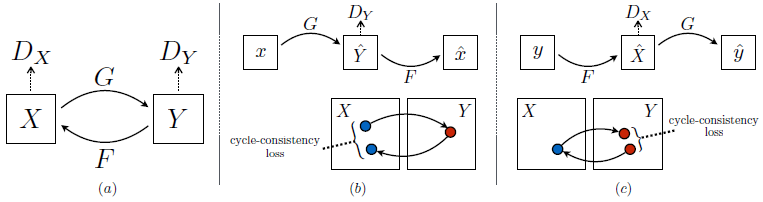
a) The model contains $2$ mapping functions $G: X \to Y$ and $F: Y \to X$, and associated adversarial discriminators $D_X$ and $D_Y$.

$D_Y$ encourages $G$ to translate $X$ into outputs indistinguishable from domain $Y$, and vice versa for $D_X$ and $F$.

For the purpose of regularizing the mappings, $2$ cycle-consistency losses are introduced, which capture the intuition that if we translate one domain to the other and back again, we should arrive at where we started.

b) Forward cycle-consistency loss: $x \to G\left(x\right) \to F\left(G\left(x\right)\right) \approx x$, and

c) Backward cycle-consistency loss: $y \to F\left(y\right) \to G\left(F\left(y\right)\right) \approx y$

Related Work

A) Generative Adversarial Networks (GANs)

1. GANs have achieved splendid results in image generation [2, 3], representation learning [3, 4], image editing [5].
2. Recent methods adopt the same idea for conditional image generation applications, such as text2image [6], image inpainting [7], and future prediction [8], as well as to other domains like videos [9] and 3D data [10].
3. The key to GANs' success is the idea of an adversarial loss that forces the generated images to be, in principle, indistinguishable from real images.
4. In the CycleGAN paper, the authors adopt an adversarial loss to learn the mapping such that the translated images can't be distinguished from images in the target domain.

B) Image-to-Image Translation

1. Recent applications all involve a dataset of input-output examples to learn a parametric translation function using CNNs (e.g. [11]).
2. The approach in the CycleGAN paper builds on the "pix2pix" framework of Isola, et al., [12] which uses a conditional GAN to learn a mapping from input to output images.
3. Parallel ideas have been applied to tasks such as generating photos from sketches [13] or from attribute and semantic layouts [14], but the CycleGAN algorithm learns the mapping without paired training examples.

C) Unpaired Image-to-Image Translation

1. The goal in an unpaired setting is to relate $2$ domains: $X$ and $Y$.
2. Rosales et al. [15] proposed a Bayesian framework which includes a prior based on a patch-based Markov random field computed from a source image and a likelihood term obtained from multiple style images.
3. CoGAN [16] and cross-modal scene networks [17] use a weight-sharing strategy to learn a common representation across domains.
4. Another line of work [18, 19] encourages the input and output to share specific "content" features even though they may differ in "style".
5. Unlike the above approaches, the CycleGAN formulation does not rely on any task-specific, predefined similarity function between the input and output, nor does it assume that the input and output have to lie in the same low-dimensional embedding space.
6. This is what makes the CycleGAN method a general-purpose solution for many computer vision and graphics use cases.

D) Cycle Consistency

1. We have explained the concept of cycle-consistency above.
2. Higher-order cycle consistency has been used in $3D$ shape matching [20], dense semantic alignment [21], and depth estimation [22].
3. Zhou et al. [23] and Godard et al. [22] are most similar to the work of the CycleGAN paper, as they used a cycle consistency loss as a way of using transitivity to supervise CNN training.
4. In the CycleGAN paper, a similar loss was introduced to push $G$ and $F$ to be consistent with each other.

E) Neural Style Transfer

1. Simply put, neural style transfer is a way to perform image-to-image translation, which generates a novel image by combining the content of one image with the style of another (usually a painting), based on matching the Gram matrix statistics of pre-trained deep features. [24, 25]
2. However, the main focus of the CycleGAN paper was to learn the mapping between $2$ image collections, rather than between $2$ specific images, by trying to capture correspondences between higher-level appearance structures.

Formulation

As explained earlier, the goal of CycleGAN is to learn mapping functions between $2$ domains $X$ and $Y$ given training examples ${\left\{x_i\right\}}_{i = 1}^N$ where $x_i \in X$ and ${\left\{y_j\right\}}_{j = 1}^M$ where $y_j \in Y$.

Let's denote the distributions as $x ~ p_{data}\left(x\right)$ and $y ~ p_{data}\left(y\right)$.

The model includes $2$ mappings $G: X \to Y$ and $F: Y \to X$.

Also, $2$ adversarial discriminators $D_X$ and $D_Y$ are introduced, where $D_X$ aims to distinguish between images $\left\{x\right\}$ and translated images $\left\{F\left(y\right)\right\}$; similarly, $D_Y$ aims to discriminate between $\left\{y\right\}$ and $\left\{G\left(x\right)\right\}$.

Two kinds of losses are made use of -

✪ Adversarial losses - for matching the distribution of generated images to the data distribution in the target domain, and

✪ Cycle-Consistency losses - to prevent the learned mappings $G$ and $F$ from contradicting each other.

I) Adversarial Loss

➢ Adversarial losses are applied to both mapping functions:
➢ For the mapping function $G: X \to Y$ and its discriminator $D_Y$, we can express the objective as:

${ℒ}_{GAN }\left(G, D_Y, X, Y\right) = {\mathbb{E}}_{y ~ p_{data}\left(y\right)}\left[\log D_Y\left(y\right)\right] + {\mathbb{E}}_{x ~ p_{data}\left(x\right)}\left[\log \left(1 - D_Y\left(G\left(x\right)\right)\right)\right]$

➢ Here, $G$ tries to generate images $G\left(x\right)$ that look similar to images from domain $Y$, while $D_Y$ aims to distinguish between translated samples $G\left(x\right)$ and real samples $y$.

➢ $G$ aims to minimize this objective against an adversary $D$ that tries to maximize it, i.e., $mi{n}_G ma{x}_{D_Y} {ℒ}_{GAN}\left(G, D_Y, X, Y\right)$

➢ Similarly, the adversarial loss for the mapping function $F: Y \to X$ and its discriminator $D_X$ is:

$mi{n}_F ma{x}_{D_X} {ℒ}_{GAN}\left(F, D_X, Y, X\right)$

II) Cycle-Consistency Loss

➢ For each image $x$ from domain $X$, the image translation cycle should be able to bring $x$ back to the original image, i.e. $x \to G\left(x\right) \to F\left(G\left(x\right)\right) \approx x$.

This is called forward cycle-consistency.

➢ Equivalently, for each image $y$ from domain $Y$, $G$ and $F$ should also satisfy backward cycle-consistency: $y \to F\left(y\right) \to G\left(F\left(y\right)\right) \approx y$.

➢ The cycle consistency loss can thus, be defined as:

${ℒ}_{cyc}\left(G, F\right) = {\mathbb{E}}_{x ~ p_{data}\left(x\right)}\left[\parallel F\left(G\left(x\right)\right) - x {\parallel }_1\right] + {\mathbb{E}}_{y ~ p_{data}\left(y\right)}\left[\parallel G\left(F\left(y\right)\right) - y {\parallel }_1\right]$

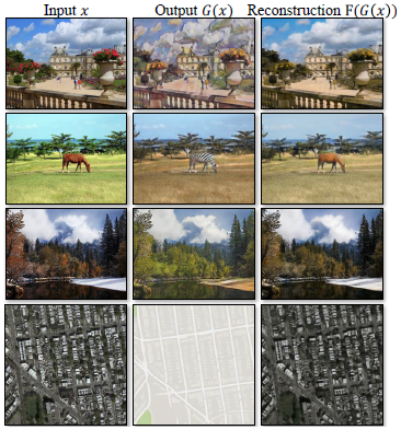
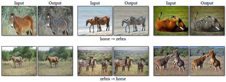
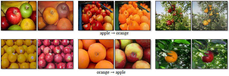
The above image shows the input images $x$, output images $G\left(x\right)$ and the reconstructed images $F\left(G\left(x\right)\right)$ from various experiments.

III) Full Objective Function

➢ The full objective function can be spread out as:

$ℒ\left(G, F, D_X, D_Y\right) = {ℒ}_{GAN}\left(G, D_Y, X, Y\right) +\hspace{0.17em}{ℒ}_{GAN}\left(F, D_X, Y, X\right) + \lambda L_{cyc}\left(G,F\right)$,

where $\lambda$ controls the relative importance of the $2$ objectives.

➢ The aim is to solve the following:

$G^{✱}, F^{✱} = arg \underset{G, F}{min} \underset{D_x, D_y}{max} ℒ\left(G, F, D_X, D_Y\right)$

IV) Model Implementation

➢ A CycleGAN is made up of $2$ architectures - a generator and a discriminator.

➢ The generator architecture is used to create $2$ models, Generator A and Generator B.

➢ The discriminator architecture is used to create another $2$ models, Discriminator A and Discriminator B.

A) Generator architecture

⚫ The generator network is akin to an autoencoder network - it takes in an image and outputs another image.

⚫ It has $2$ parts: an encoder and a decoder.

⚫ The encoder contains convolutional layers with downsampling capabilities and transforms an input of shape $\left(128, 128, 3\right)$ to an internal representation.

⚫ The decoder contains $2$ upsampling blocks and a final convolutional layer, which transforms the internal representation to an output of shape $\left(128, 128, 3\right)$.

⚫ The generator network contains the following $4$ blocks:
➜ The convolutional block
➜ The residual block
➜ The upsampling block
➜ The final convolutional layer

The convolutional block

❂ The convolutional block contains a $2D$ convolutional layer, followed by an instance normalization layer, and ReLU as the activation function.

❂ The generator network contains $3$ convolutional blocks.

The residual block

❂ The residual block contains two $2D$ convolutional layers.

❂ Both layers are followed by a batch normalization layer with a momentum value of $0.8$

❂ The generator network contains $6$ residual blocks.

❂ The addition layer which is the concluding layer of this block calculates the sum of the input tensor to the block and the output of the last batch normalization layer.

The upsampling block

❂ The upsampling block contains a transpose $2D$ convolutional layer and uses ReLU as the activation function.

❂ There are $2$ upsampling blocks in the generator network.

The final convolutional layer

❂ The last layer is a $2D$ convolutional layer that uses Tanh as the activation function.

❂ It generates an image of shape $\left(128, 128, 3\right)$.

B) Discriminator Architecture

⚫ The architecture of the discriminator network is similar to that of the discriminator in a PatchGAN network.

⚫ It is a deep convolutional neural network and contains several convolutional blocks.

⚫ What it basically does is, take in an image having shape $\left(128, 128, 3\right)$ and predicts whether the image is real or fake.

⚫ It contains several ZeroPadding2D layers too.

⚫ The discriminator network returns a tensor of shape $\left(7, 7, 1\right)$.

C) The Training Objective Function

⚫ CycleGANs have a training objective function which we need to minimize in order to train the model.

⚫ The loss function is a weighted sum of $2$ losses:

1. Adversarial loss
2. Cycle-consistency loss

Please refer to the Formulation section above to learn about these loss functions.

Results

I) Evaluation Metric (FCN Score)

➤ The FCN score was chosen as an automatic quantitative meausre which does not require human experiments and supervision (like in Amazon Mechanical Turk perceptual studies)

➤ The FCN score from [12] was adopted, and used to evaluate the performance of the CycleGAN on the Cityscapes labels $\to$ photo task.

➤ The FCN metric evaluates how interpretable the generated photos are according to an off-the-shelf semantic segmentation algorithm (the fully connected network, FCN, from [11]).

➤ The FCN predicts a label map for a generated photo.

➤ This label map can then be compared against the input ground truth labels using standard semantic segmentation metrics (per-pixel accuracy, per-class accuracy and mean class Intersection-Over-Union (Class IOU)).

➤ The point is that, if we generate a photo from a label map of "bird on the tree", then we have succeeded if the FCN applied to the generated photo detects "bird on the tree".

II) Baselines

➤ Different models and architectures were trained alongside the CycleGAN so that a comprehensive performance evaluation could be made.

➤ The models that were tested are as follows:
➡ CoGAN [16]
➡ SimGAN [18]
➡ Feature loss + GAN
➡ BiGAN / ALI [26]
➡ pix2pix [12]

III) Comparison against the baselines

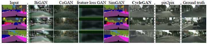
The image above illustrates the different methods for mapping labels $\leftrightarrow$ photos trained on Cityscapes images.

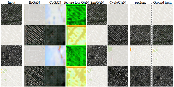
This image depicts the different methods for mapping aerial photos $\leftrightarrow$ maps on Google Maps.

It is obvious from the renderings above that the authors were unable to achieve credible results with any of the baselines.

Their CycleGAN method on the other hand, was able to produce translations that were often of similar quality to the fully supervised pix2pix.

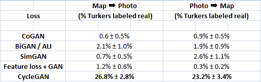
Table 1: AMT "real vs fake" test on maps $\leftrightarrow$ aerial photos at $256$ x $256$ resolution.

Table 1 reports performance regarding the AMT perceptual realism task.

Here, we see that the CycleGAN method can fool participants on around a quarter of trials, in both the maps $\to$ aerials photos direction and the aerial photos $\to$ maps direction at $256$ x $256$ resolution.

All the baselines almost never fooled participants.

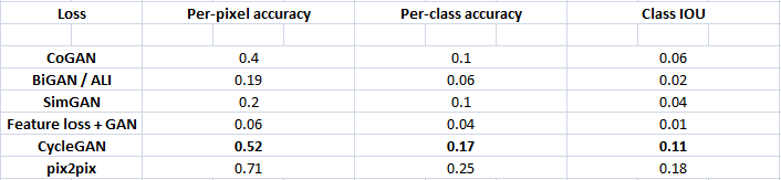
Table 2: FCN-scenes for different methods, evaluated on Cityscapes labels $\to$ photo.

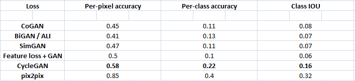
Table 3: Classification performance of photo $\to$ labels for different methods on cityscapes.

Table 2 evaluates the perfomance of the labels $\to$ photo task on the Cityscapes and Table 3 assesses the opposite mapping (photos $\to$ labels).

In both cases, the CycleGAN method again outperforms the baselines.

IV) Additional results on paired datasets

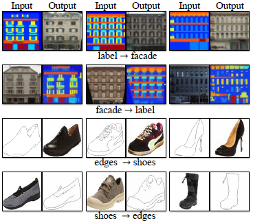
Shown above are example results of CycleGAN on paired datasets used in "pix2pix", such as architectural labels $\leftrightarrow$ photos (from the CMP Facade Database) and edges $\leftrightarrow$ shoes (from the UT Zappos50K dataset).

The image quality of the CycleGAN results is close to those produced by the fully supervised pix2pix while the former method learns the mapping without paired supervision.

Implementation of CycleGAN in Keras

The entire working code of the CycleGAN model adds up to around 400 lines of code in Python, which we obviously won't manifest here.

But, we will show you how the Residual block, the Generator and the Discriminator networks are implemented, using the Keras framework.

Let's import all the required libraries first:

import time
import numpy as np
import tensorflow as tf
import matplotlib.pyplot as plt
import PIL

from glob import glob
from keras import Input, Model
from keras.callbacks import TensorBoard
from keras.layers import Conv2D, BatchNormalization, Activation
from keras.layers import Add, Conv2DTranspose, ZeroPadding2D, LeakyReLU
from keras.optimizers import Adam
from imageio import imread
from skimage.transform import resize
from keras_contrib.layers.normalization.instancenormalization Import InstanceNormalization

I) Residual Block

def residual_block(x):

    """
    Residual block
    """
    
    res = Conv2D(filters = 128, kernel_size = 3, strides = 1, padding = "same")(x)
    res = BatchNormalization(axis = 3, momentum = 0.9, epsilon = 1e-5)(res)
    res = Activation('relu')(res)
    res = Conv2D(filters = 128, kernel_size = 3, strides = 1, padding = "same")(res)
    res = BatchNormalization(axis = 3, momentum = 0.9, epsilon = 1e-5)(res)
    
    return Add()([res, x])
    

II) Generator Network

def build_generator():

    """
    Creating a generator network with the hyperparameters defined below
    """
    
    input_shape = (128, 128, 3)
    residual_blocks = 6
    input_layer = Input(shape = input_shape)
    
    
    ## 1st Convolutional Block
    x = Conv2D(filters = 32, kernel_size = 7, strides = 1, padding = "same")(input_layer)
    x = InstanceNormalization(axis = 1)(x)
    x = Activation("relu")(x)
    
    ## 2nd Convolutional Block
    x = Conv2D(filters = 64, kernel_size = 3, strides = 2, padding = "same")(x)
    x = InstanceNormalization(axis = 1)(x)
    x = Activation("relu")(x)
    
    ## 3rd Convolutional Block
    x = Conv2D(filters = 128, kernel_size = 3, strides = 2, padding = "same")(x)
    x = InstanceNormalization(axis = 1)(x)
    x = Activation("relu")(x)
    
    
    ## Residual blocks
    for _ in range(residual_blocks):
      x = residual_block(x)
      
    
    ## 1st Upsampling Block
    x = Conv2DTranspose(filters = 64, kernel_size = 3, strides = 2, padding = "same", 
                        use_bias = False)(x)
    x = InstanceNormalization(axis = 1)(x)
    x = Activation("relu")(x)
    
    ## 2nd Upsampling Block
    x = Conv2DTranspose(filters = 32, kernel_size = 3, strides = 2, padding = "same", 
                        use_bias = False)(x)
    x = InstanceNormalization(axis = 1)(x)
    x = Activation("relu")(x)
    
    ## Last Convolutional Layer
    x = Conv2D(filters = 3, kernel_size = 7, strides = 1, padding = "same")(x)
    output = Activation("tanh")(x)
    
    
    model = Model(inputs = [input_layer], outputs = [output])
    return model

III) Discriminator Network

def build_discriminator():

    """
    Create a discriminator network using the hyperparameters defined below
    """
    
    input_shape = (128, 128, 3)
    hidden_layers = 3
    
    input_layer = Input(shape = input_shape)
    
    x = ZeroPadding2D(padding = (1, 1))(input_layer)
    
    
    ## 1st Convolutional Block
    x = Conv2D(filters = 64, kernel_size = 4, strides = 2, padding = "valid")(x)
    x = LeakyReLU(alpha = 0.2)(x)
    x = ZeroPadding2D(padding = (1, 1))(x)
    
    ## 3 Hidden Convolutional Blocks
    for i in range(1, hidden_layers + 1):
      x = Conv2D(filters = 2 ** i * 64, kernel_size = 64, strides = 2, padding = "valid")(x)
      x = InstanceNormalization(axis = 1)(x)
      x = LeakyReLU(alpha = 0.2)(x)
      x = ZeroPadding2D(padding = (1, 1))(x)
      
    
    ## Last Convolutional Layer
    output = Conv2D(filters = 1, kernel_size = 4, strides = 1, activation = "sigmoid")(x)
    
    model = Model(inputs = [input_layer], outputs = [output])
    return model

Bonus:

You can find the entire code for the CycleGAN model at this link.

Applications

The CycleGAN method is demonstrated on several use cases where paired training data does not exist.

It was observed by the authors that translations on training data are often more appealing than those on test data.

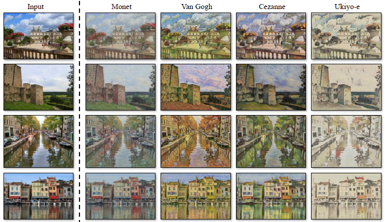
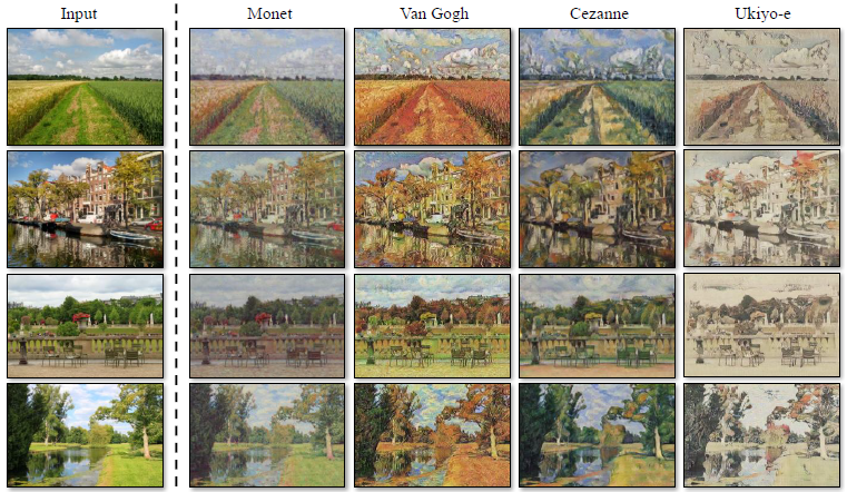
▶ Collection Style transfer

1. The model was trained on landscape photographs from Flickr and WikiArt.
2. Unlike recent work on "neural style transfer", this method learns to mimic the style of an entire collection of artworks, rather than transferring the style of a single selected piece of art.
3. Therefore, we can learn to generate photos in the style of, e.g. Van Gogh, rather than just in the style of Starry Night.
4. The size of the dataset for each artist / style was $526$, $1073$, $400$, and $563$ for Cezanne, Monet, Van Gogh, and Ukiyo-e.

▶ Object Transfiguration

1. The model is trained to translate one object class from ImageNet to another (each class contains around $1000$ training images).
2. Campbell et al. [27] proposed a subspace model to translate one object into another, belonging to the same category, while the CycleGAN method focuses on object transfiguration between $2$ visually similar categories.

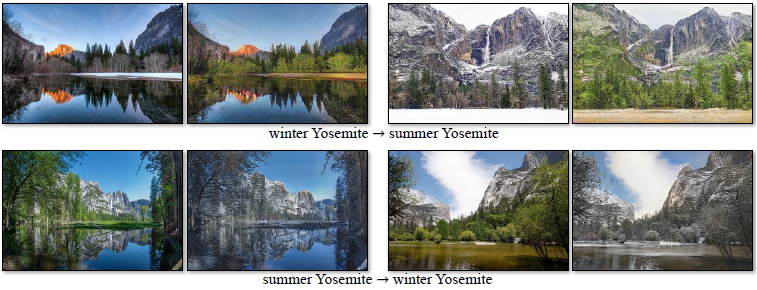
▶ Season transfer

The model was trained on $854$ winter photos and $1273$ summer photos of Yosemite, downloaded from Flickr.

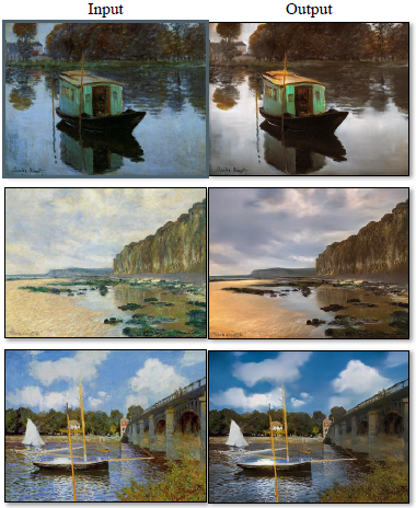
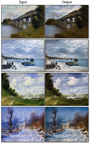
▶ Photo generation from paintings

The images below portray the relatively successful results on mapping Monet's paintings to a photographic style.

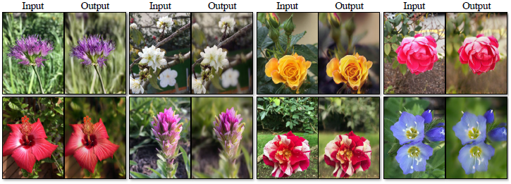
▶ Photo enhancement

1. The CycleGAN method can also be used to generate photos with shallower depth of field (DoF).
2. The model was trained on flower photos obtained from Flickr.
3. The source domain consists of flower photos taken by smartphones, which usually have deep DoF due to a small aperture.
4. The target contains photos captured by DSLR with a larger aperture.
5. It was noted that the model successfully generated photos with shallower DoF from the photos taken by smartphones.

References

1. Isola, et al. (2018), "Unpaired Image-to-Image Translation using Cycle-Consistent Adversarial Networks"
2. Chintala, et al. (2015), "Deep Generative Image Models using a Laplacian Pyramid of Adversarial Networks"
3. Chintala, et al. (2015), "Unsupervised Representation Learning with Deep Convolutional GANs"
4. Goodfellow, et al. (2016), "Improved Techniques for Training GANs"
5. Efros, et al. (2016), "Generative Visual Manipulation of the Natural Image Manifold"
6. Reed, et al. (2016), "Generative Adversarial Text to Image Synthesis"
7. Efros, et al. (2016), "Context Encoders: Feature Learning by Inpainting"
8. LeCun, et al. (2016), "Deep multi-scale video prediction beyond mean square error"
9. Vondrick, et al. (2016), "Generating videos with scene dynamics"
10. Tenenbaum, et al. (2016), "Learning a probabilistic latent space of object shapes via 3D generative-adversarial modeling"
11. Darrell, et al. (2015), "Fully convolutional networks for semantic segmentation"
12. Isola, et al. (2017), "Image-to-image translation with conditional adversarial networks"
13. Hays, et al. (2016), "Controlling deep image synthesis with sketch and color"
14. Erdem, et al. (2016), "Learning to generate images of outdoor scenes from attributes and semantic layouts"
15. Rosales, et al. (2003), "Unsupervised Image Translation"
16. Liu, et al. (2016), "Coupled generative adversarial networks"
17. Vondrick, et al. (2016), "Cross-modal scene networks"
18. Pfister, et al. (2017), "Learning from simulated and unsupervised images through adversarial learning"
19. Wolf, et al. (2017), "Unsupervised cross-domain image generation"
20. Huang, et al. (2013), "Consistent shape maps via semidefinite programming"
21. Efros, et al. (2015), "Flowweb: Joint image set alignment by weaving consistent, pixel-wise correspondences"
22. Godard, et al. (2017), "Unsupervised monocular depth estimation with left-right consistency"
23. Efros, et al. (2016), "Learning dense correspondence via 3D-guided cycle consistency"
24. Gatys, et al. (2016), "Image style transfer using convolutional neural networks"
25. Johnson, et al. (2016), "Perceptual losses for real-time style transfer and super-resolution"
26. Poole, et al. (2017), "Adversarially learned inference"
27. Campbell, et al. (2015), "Modeling object appearance using context-conditioned component analysis"

So that was it, dear reader. I hope you enjoyed the article above and learnt how CycleGANs can generate realistic renditions of paintings without using paired training data.

Please comment below to let me know your views on this post, and also, any doubts that you might have.

Follow me on LinkedIn and Medium to get updates on more articles ☺ .