
Open-Source Internship opportunity by OpenGenus for programmers. Apply now.
Reading time: 30 minutes
In this article, we will develop and train a convolutional neural network (CNN) in Python using TensorFlow for digit recognifition with MNIST as our dataset. We will give an overview of the MNIST dataset and the model architecture we will work on before diving into the code.
What is MNIST data?
MNIST ("Modified National Institute of Standards and Technology") is the de facto “hello world” dataset of computer vision. Since its release in 1999, this classic dataset of handwritten images has served as the basis for benchmarking classification algorithms. As new machine learning techniques emerge, MNIST remains a reliable resource for researchers and learners alike.
MNIST is a dataset consisting of 60,000+ images of handwritten digits for training and another 10,000 for testing. Each training example comes with an associated label (0 to 9) indicating what digit it is. Each digit will be a black and white image of 28 X 28 pixels.

Architecture of CNN
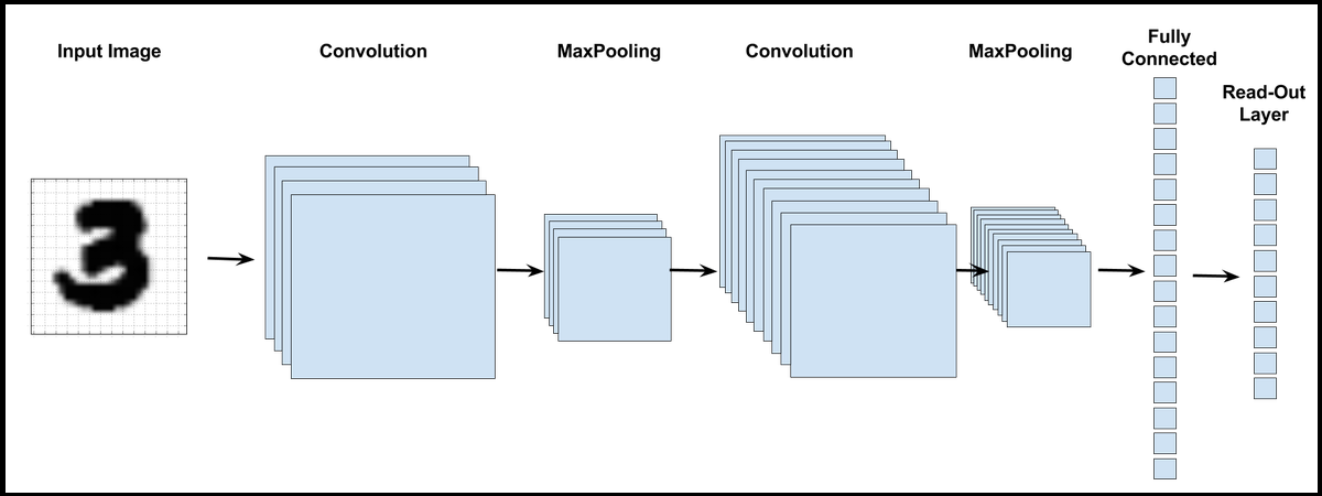 A convolutional neural network is different from a standard artificial neural network, and may involve convolutional, pooling, fully connected and softmax layers. Let's understand each of these layers.
Tensorflow implementation
STEP 1: Importing Tensorflow:
import tensorflow as tf
STEP 2: Importing the dataset:
The MNIST data is stored in the Tensorflow library, we can just import it from there:
from tensorflow.examples.tutorials.mnist import input_data
mnist = input_data.read_data_sets("/tmp/data/", one_hot=False)
STEP 3: Initializing the parameters
We will first need to initialize a few parameters, along with x and y:
n_classes = 10
batch_size = 128

x = tf.placeholder('float', [None, 784])
y = tf.placeholder('float')

keep_rate = 0.8
keep_prob = tf.placeholder(tf.float32)
STEP 4: Initializing the weights and bias parameters
We'll define a weight and bias dictionary in this step. The dimensions for each layer need to be specified, in order to maintain consistency in the model. We use tf.random.normal in order to randomize the values initially.
For the convolutional layers, we specify 5x5 filters. Next, we define the number of input and output features. For example, for W_conv2 ,the weights will have values [5,5,1,32]. We do similar definition for the biases as well. The fully connected layer will have 1024 parameters to train.
weights = {'W_conv1':tf.Variable(tf.random_normal([5,5,1,32])),
               'W_conv2':tf.Variable(tf.random_normal([5,5,32,64])),
               'W_fc':tf.Variable(tf.random_normal([7*7*64,1024])),
               'out':tf.Variable(tf.random_normal([1024, n_classes]))}

biases = {'b_conv1':tf.Variable(tf.random_normal([32])),
               'b_conv2':tf.Variable(tf.random_normal([64])),
               'b_fc':tf.Variable(tf.random_normal([1024])),
               'out':tf.Variable(tf.random_normal([n_classes]))}
STEP 5: Reshaping the input feature vector:
The input feature vector, x, will need to be reshaped in order to fit the standard tensorflow syntax. Tensorflow takes 4D data as input for models, hence we need to specify it in 4D format. Each training example will be of 28X28 pixels. Hence, the tensorflow reshape function needs to be specified as:
x = tf.reshape(x, shape=[-1, 28, 28, 1])
STEP 6: Convolutional layer
 Convolutional layer is generally the first layer of a CNN. It calculates the element wise product of the image matrix, and a filter. In the above example, the image is a 5 x 5 matrix and the filter going over it is a 3 x 3 matrix. A convolution operation takes place between the image and the filter and the convolved feature is generated. The convoluted feature shown in the gif is the output of a convolutional layer.
The function defined below will take the feature vector and weight vector as input and add a convolutional layer to our tensorflow model accordingly.
def conv2d(x, W):
    return tf.nn.conv2d(x, W, strides=[1,1,1,1], padding='SAME')
Here's how we'll call the function later on in the code:
 conv1 = tf.nn.relu(conv2d(x, weights['W_conv1']) + biases['b_conv1']) #First conv layer

 conv2 = tf.nn.relu(conv2d(conv1, weights['W_conv2']) + biases['b_conv2']) #Second conv layer
STEP 7: Pooling layer
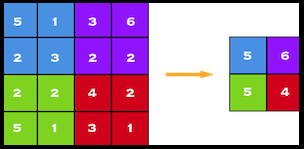 Pooling layers are generally added after a convolutional layer, to reduce the dimensions of our data. A pooling window size is selected, and all the values in there will be replaced by the maximum, average or some other value. Max Pooling, one of the most common pooling techniques, may be demonstrated as follows:
The following function is a maxpool function, taking the feature vector as input and adding a max-pooling layer to our model. The window size and strides are defined as shown.
def maxpool2d(x):
    #                        size of window         movement of window
    return tf.nn.max_pool(x, ksize=[1,2,2,1], strides=[1,2,2,1], padding='SAME')
Here's how we'll call the function later on in the code:
conv1 = maxpool2d(conv1)

conv2 = maxpool2d(conv2)
STEP 8: Fully connected layer
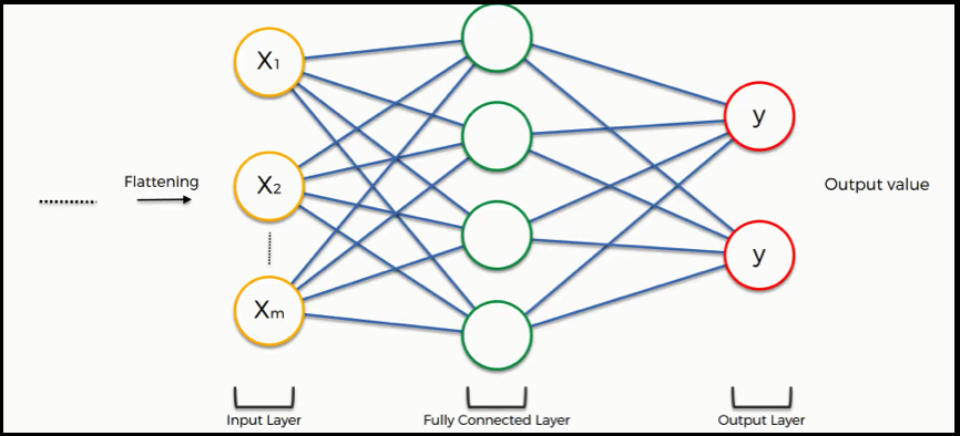
Now that our convolutional and pooling layers have reduced complexity of the data, we can use a regular fully connected layer in order to determine the true relation that our parameters have on labels. In order to classify the images as one label from 0 to 9, such a layer is needed. The data is flattenned to make it linear. These layers generally use the RELU activation function.
These lines are used to implement the fully connected layer in our neural network. Dropout is a regularization method used to prevent overfitting.
fc = tf.reshape(conv2,[-1, 7*7*64])
fc = tf.nn.relu(tf.matmul(fc, weights['W_fc'])+biases['b_fc'])
fc = tf.nn.dropout(fc, keep_rate)
STEP 9: Softmax output layer
Softmax is an output layer function which is used for multi-class classification problems. As we need an output layer which can classify a digit as either from 0 to 9, softmax function can be used to classify it to either of the 10 classes.

# Here we make use of a Softmax function and compare the result with the y label.
cost = tf.reduce_mean( tf.nn.softmax_cross_entropy_with_logits(prediction,y) )
STEP 10: Optimizing and Training:
An optimizer is used to refine the weights and biases, i.e. the parameters of the model so that the loss function is minimized. We'll use the 'Adam' Optimizer for our model.
optimizer = tf.train.AdamOptimizer().minimize(cost)

with tf.Session() as sess:
        sess.run(tf.initialize_all_variables())

        for epoch in range(hm_epochs):
            epoch_loss = 0
            for _ in range(int(mnist.train.num_examples/batch_size)):
                epoch_x, epoch_y = mnist.train.next_batch(batch_size)
                _, c = sess.run([optimizer, cost], feed_dict={x: epoch_x, y: epoch_y})
                epoch_loss += c

            print('Epoch', epoch, 'completed out of',hm_epochs,'loss:',epoch_loss)

        correct = tf.equal(tf.argmax(prediction, 1), tf.argmax(y, 1))
STEP 11: Accuracy of the model:
In this step, we find the accuracy of the model in order to determine how well our model does on test data.
accuracy = tf.reduce_mean(tf.cast(correct, 'float'))
print('Accuracy:',accuracy.eval({x:mnist.test.images, y:mnist.test.labels}))
Complete Source Code
import tensorflow as tf
from tensorflow.examples.tutorials.mnist import input_data
mnist = input_data.read_data_sets("/tmp/data/", one_hot = True)

n_classes = 10
batch_size = 128

x = tf.placeholder('float', [None, 784])
y = tf.placeholder('float')

keep_rate = 0.8
keep_prob = tf.placeholder(tf.float32)

def conv2d(x, W):
    return tf.nn.conv2d(x, W, strides=[1,1,1,1], padding='SAME')

def maxpool2d(x):
    #                        size of window         movement of window
    return tf.nn.max_pool(x, ksize=[1,2,2,1], strides=[1,2,2,1], padding='SAME')


def convolutional_neural_network(x):
    weights = {'W_conv1':tf.Variable(tf.random_normal([5,5,1,32])),
               'W_conv2':tf.Variable(tf.random_normal([5,5,32,64])),
               'W_fc':tf.Variable(tf.random_normal([7*7*64,1024])),
               'out':tf.Variable(tf.random_normal([1024, n_classes]))}

    biases = {'b_conv1':tf.Variable(tf.random_normal([32])),
               'b_conv2':tf.Variable(tf.random_normal([64])),
               'b_fc':tf.Variable(tf.random_normal([1024])),
               'out':tf.Variable(tf.random_normal([n_classes]))}

    x = tf.reshape(x, shape=[-1, 28, 28, 1])

    conv1 = tf.nn.relu(conv2d(x, weights['W_conv1']) + biases['b_conv1'])
    conv1 = maxpool2d(conv1)

    conv2 = tf.nn.relu(conv2d(conv1, weights['W_conv2']) + biases['b_conv2'])
    conv2 = maxpool2d(conv2)

    fc = tf.reshape(conv2,[-1, 7*7*64])
    fc = tf.nn.relu(tf.matmul(fc, weights['W_fc'])+biases['b_fc'])
    fc = tf.nn.dropout(fc, keep_rate)

    output = tf.matmul(fc, weights['out'])+biases['out']

    return output

def train_neural_network(x):
    prediction = convolutional_neural_network(x)
    cost = tf.reduce_mean( tf.nn.softmax_cross_entropy_with_logits(prediction,y) )
    optimizer = tf.train.AdamOptimizer().minimize(cost)

    hm_epochs = 10
    with tf.Session() as sess:
        sess.run(tf.initialize_all_variables())

        for epoch in range(hm_epochs):
            epoch_loss = 0
            for _ in range(int(mnist.train.num_examples/batch_size)):
                epoch_x, epoch_y = mnist.train.next_batch(batch_size)
                _, c = sess.run([optimizer, cost], feed_dict={x: epoch_x, y: epoch_y})
                epoch_loss += c

            print('Epoch', epoch, 'completed out of',hm_epochs,'loss:',epoch_loss)

        correct = tf.equal(tf.argmax(prediction, 1), tf.argmax(y, 1))

        accuracy = tf.reduce_mean(tf.cast(correct, 'float'))
        print('Accuracy:',accuracy.eval({x:mnist.test.images, y:mnist.test.labels}))

train_neural_network(x)