
Open-Source Internship opportunity by OpenGenus for programmers. Apply now.
Reading time: 15 minutes | Coding time: 5 minutes
In this article, we have explored the time and space complexity of Insertion Sort along with two optimizations. Before going into the complexity analysis, we will go through the basic knowledge of Insertion Sort.
In short:
- The worst case time complexity of Insertion sort is
O(N^2) - The average case time complexity of Insertion sort is
O(N^2) - The time complexity of the best case is
O(N). - The space complexity is
O(1)
What is Insertion Sort?
Insertion sort is one of the intutive sorting algorithm for the beginners which shares analogy with the way we sort cards in our hand.
As the name suggests, it is based on "insertion" but how?
An array is divided into two sub arrays namely sorted and unsorted subarray.
How come there is a sorted subarray if our input in unsorted?
The algorithm is based on one assumption that a single element is always sorted.
Hence, the first element of array forms the sorted subarray while the rest create the unsorted subarray from which we choose an element one by one and "insert" the same in the sorted subarray. The same procedure is followed until we reach the end of the array.
In each iteration, we extend the sorted subarray while shrinking the unsorted subarray.
Working Principle
- Compare the element with its adjacent element.
- If at every comparison, we could find a position in sorted array where the element can be inserted, then create space by shifting the elements to right and insert the element at the appropriate position.
- Repeat the above steps until you place the last element of unsorted array to its correct position.
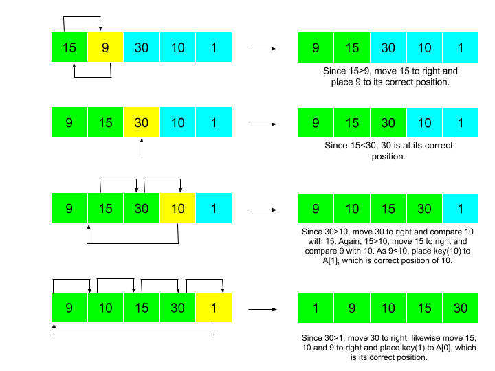
Let's take an example.
Input: 15, 9, 30, 10, 1
Expected Output: 1, 9, 10, 15, 30
The steps could be visualized as:
Pseudocode
1.    for i = 0 to n
2.        key = A[i]
3.        j = i - 1
4.        while j >= 0 and A[j] > key
5.            A[j + 1] = A[j]
6.            j = j - 1
7.        end while
8.    A[j + 1] = key
9.    end for
Complexity
- Worst case time complexity:
Θ(n^2) - Average case time complexity:
Θ(n^2) - Best case time complexity:
Θ(n) - Space complexity:
Θ(1)
Implementation
// C++ program for insertion sort
#include <bits/stdc++.h>
using namespace std;
/* Function to sort an array using insertion sort*/
void insertionSort(int arr[], int n)
{
    int i, k, j;
    for (i = 1; i < n; i++)
    {
        k = arr[i];
        j = i - 1;
        /*shifting elements of arr[0..i-1] towards right
		  if are greater than k */
        while (j >= 0 && arr[j] > k)
        {
            arr[j + 1] = arr[j];
            j = j - 1;
        }
        arr[j + 1] = k;
    }
}
int main()
{
    int n,i;
    // size of array
    cin>>n;
    int arr[n];
    for (i = 0; i < n; i++)
        cin >> arr[i];
    // input the array
    insertionSort(arr, n);
	// sort the array
    for (i = 0; i < n; i++)
        cout << arr[i] << " ";
    cout << endl;
    // print the array
    return 0;
}
Complexity Analysis for Insertion Sort
We examine Algorithms broadly on two prime factors, i.e.,
-
Running Time
Running Time of an algorithm is execution time of each line of algorithm
As stated, Running Time for any algorithm depends on the number of operations executed. We could see in the Pseudocode that there are precisely 7 operations under this algorithm. So, our task is to find the Cost or Time Complexity of each and trivially sum of these will be the Total Time Complexity of our Algorithm.
We assume Cost of each i operation as C i where i ∈ {1,2,3,4,5,6,8} and compute the number of times these are executed. Therefore the Total Cost for one such operation would be the product of Cost of one operation and the number of times it is executed.
We could list them as below:
| Cost of line | No. of times it is run |
|---|---|
| C1 | n |
| C2 | n - 1 |
| C3 | n - 1 |
| C4 | Σ n - 1j = 1(tj) |
| C5 | Σ n - 1j = 1 (tj - 1) |
| C6 | Σ n - 1j = 1(tj - 1) |
| C8 | n - 1 |
Then Total Running Time of Insertion sort (T(n)) = C1 * n + ( C2 + C3 ) * ( n - 1 ) + C4 * Σ n - 1j = 1( t j ) + ( C5 + C6 ) * Σ n - 1j = 1( t j ) + C8 * ( n - 1 )
-
Memory usage
Memory required to execute the Algorithm.
As we could note throughout the article, we didn't require any extra space. We are only re-arranging the input array to achieve the desired output. Hence, we can claim that there is no need of any auxiliary memory to run this Algorithm. Although each of these operation will be added to the stack but not simultaneoulsy the Memory Complexity comes out to be O(1)
Best Case Analysis
In Best Case i.e., when the array is already sorted, tj = 1
Therefore,T( n ) = C1 * n + ( C2 + C3 ) * ( n - 1 ) + C4 * ( n - 1 ) + ( C5 + C6 ) * ( n - 2 ) + C8 * ( n - 1 )
which when further simplified has dominating factor of n and gives T(n) = C * ( n ) or O(n)
Worst Case Analysis
In Worst Case i.e., when the array is reversly sorted (in descending order), tj = j
Therefore,T( n ) = C1 * n + ( C2 + C3 ) * ( n - 1 ) + C4 * ( n - 1 ) ( n ) / 2 + ( C5 + C6 ) * ( ( n - 1 ) (n ) / 2 - 1) + C8 * ( n - 1 )
which when further simplified has dominating factor of n2 and gives T(n) = C * ( n 2) or O( n2 )
Average Case Analysis
Let's assume that tj = (j-1)/2 to calculate the average case
Therefore,T( n ) = C1 * n + ( C2 + C3 ) * ( n - 1 ) + C4/2 * ( n - 1 ) ( n ) / 2 + ( C5 + C6 )/2 * ( ( n - 1 ) (n ) / 2 - 1) + C8 * ( n - 1 )
which when further simplified has dominating factor of n2 and gives T(n) = C * ( n 2) or O( n2 )
Can we optimize it further?
Searching for the correct position of an element and Swapping are two main operations included in the Algorithm.
-
We can optimize the searching by using Binary Search, which will improve the searching complexity from O(n) to O(log n) for one element and to n * O(log n) or O(n log n) for n elements.
But since it will take O(n) for one element to be placed at its correct position, n elements will take n * O(n) or O(n2) time for being placed at their right places. Hence, the overall complexity remains O(n2). -
We can optimize the swapping by using Doubly Linked list instead of array, that will improve the complexity of swapping from O(n) to O(1) as we can insert an element in a linked list by changing pointers (without shifting the rest of elements).
But since the complexity to search remains O(n2) as we cannot use binary search in linked list. Hence, The overall complexity remains O(n2).
Therefore, we can conclude that we cannot reduce the worst case time complexity of insertion sort from O(n2) .
Advantages
- Simple and easy to understand implementation
- Efficient for small data
- If the input list is sorted beforehand (partially) then insertions sort takes
O(n+d)where d is the number of inversions - Chosen over bubble sort and selection sort, although all have worst case time complexity as
O(n^2) - Maintains relative order of the input data in case of two equal values (stable)
- It requires only a constant amount
O(1)of additional memory space (in-place Algorithm)
Applications
- It could be used in sorting small lists.
- It could be used in sorting "almost sorted" lists.
- It could be used to sort smaller sub problem in Quick Sort.