The aim of this article is to explain the influential research paper "Intriguing properties of neural networks" by Christian Szegedy and others in simple terms so that people who are trying to break into deep learning can have a better idea of this wonderful paper by referring this article.

Introduction

Deep learning models are one of the most powerful models for both vision and speech recognition. Deep learning models has many layers which are parallel to each other and have non linear relationships. The main property of deep learning is that it is able to identify and extract the features automatically through back propagation. Thus the model acts like a black box which works really well. But, we do not know or have control of what is happening inside the model. Thus it is very difficult to interpret the model and it can also have counter intuitive properties. In this paper, we will discuss two such counter intuitive properties in the deep neural network.

The first property is the semantic meaning of individual unit. In other words, what kind of features do these units react to or activate upon. The second one is related to stability of the neural network with respect to small variations in their inputs (perterbation).

Framework

Throughout this network, we represent the input image by and the activation value for any particular layer is represented as .

Here, we perform multiple experiments on numerous networks and three different datasets.

1. For MNIST dataset, we use the following architectures.
   A simple neural network with one or more hidden layers and a softmax function in the final layer. We refer to this network as "FC"
   A classification model is trained on the top of the autoencoder. We refer to this as "AE"
2. The ImageNet dataset
   We refer to this as AlexNet
3. 10 M image samples from Youtube
   It is unsupervisedly trained network with over 1 billion learnable parameters. We refer to it as "QuocNet"

Unit level inspection

In traditional computer vision techniques, we used simple feature extraction by using basic matplotlib library using specific coding. For example we can extract a specif intensity of colour, specific direction of lines etc. But a deep learning model has numerous units and layers. So we cannot really identify which layer is identifying which feature and what the procedure is unless obtained individually.

Here, we define a feature vector space which we want to filter from the set of images. Now, we will use two type of feature vectors - a natural basis vector (a basis vector which has magnitude for only one direction) and a random basis vector (which has random direction). These experiments are performed on MNIST dataset on the test dataset (images priorly not seen by the model) and the results are given below.

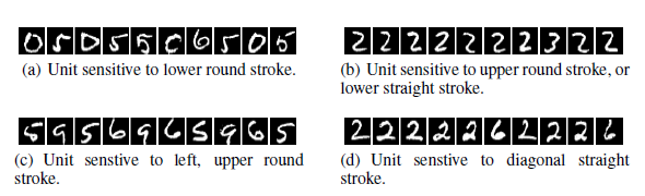
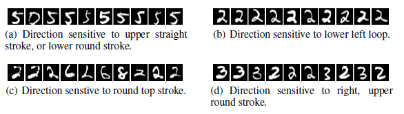
It is evident from the above results that both of these methods perform almost similar to each other. They are able to find what is required.

The experiment is repeated. But now with AlexNet dataset. It is to determine if both the vector spaces are able to capture semantic meaning within their units. The results are given below.

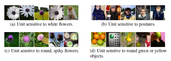
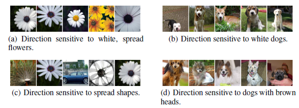
From the results, it is clear that both of these are able to perform similar in obtaining the features.

Blind spot of deep network

This earlier mentioned method helps us find what a particular unit is doing in the deep neural network. But when we consider a really deep network, it has very little help. We can use otherwise a trained model on already classified datasets to determine which features are being captured. The deep neural networks are non linear in nature. The output obtained has mostly no coherence with its input images. Each layer has different non linear activation functions and are assigned different values. This phenomenon is called non - local generalization prior. Images which are classified in one domain will not give the same results when it is viewed from a farpoint (zooming the image). These images obtained by small changes and are not able to be identified by the trained models are called adversial examples. These examples have low probability and are hard to find by the model. Many of the current computer vision frameworks use this to improve the efficiency of the model and its convergence speed. This process is called data augmentation.

This can be made analogous to hard - negative mining where we find the set of examples which are given low probability in the model but should be given high probability. The training set is trained again given more priotorization to those augmented data. We have proposed a optimization method similar to hard - negative mining.

Experimental Results

The minimum distortion function in the model has the following intriguing properties.

1. For all the three above mentioned dataset, for each sample, we have managed to generate very close, visually hard to distinguish advarsarial examples that are misclassified by the original model.
2. Cross Model generalization : a relatively large fraction of examples will be misclassified by networks trained from scratch with different hyper-parameters (number of layers, regularization or initial weights). In other words, if there is a slight modification in the original model, it produces wrong results.
3. Cross training-set generalization : a relatively large fraction of examples will be misclassified by networks trained from scratch on a disjoint training set. In other words, if there is a modification in the training dataset, they the model produces wrong classification results.

This helps us understand that training the images on adversarial data improves the generalization of the model. With MNIST dataset, we have successfully trained a two layer network with 100 layers on input layer and 100 layers on hidden layer. Usually, we don't consider output layer as a layer in the network. We have achieved a test error of just 1.2% by giving in a pool of adversarial data replacing existing data. We have used weight decay but not dropout.

For comparison, if a similar sized dataset is trained alone with weight decay, it produces 1.6% error. It can further be improved to 1.3% by careful dropout. This proves that adversarial examples decreases error. It is also observed that adding adversarial data to higher order layers has better effects than comparing to lower order layers. The examples of such generated adversarial examples are given below for MNIST dataset.

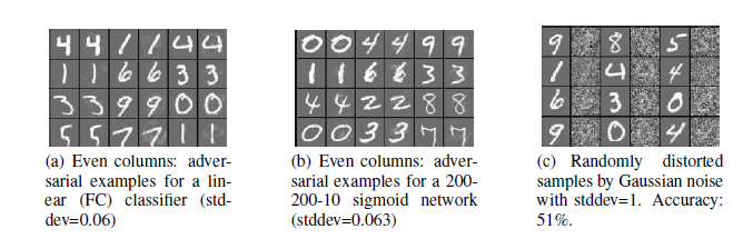
The results of the experiment performed on MNIST dataset are given below.

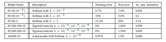
The first three model are linear models which work on pixel level with various weight decay parameters. The other three models are simple linear models (softmax) without any hidden layers. One of them have a very high learning parameter of 1. Two of these models are simple sigmoidal neural network with two hidden layers and a output layer. The last layer consists of a single layer sparse autoencoded with sigmoidal activation function and 400 nodes with a softmax classifier. Distortion is given by the below formula where the numerator represents the changes between original and changed images.

In the same experiment, we generated a set of adversarial examples and added them to the training set to measure the instances of misclassified images. The results are given below.

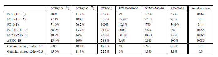
The last column shows the minimum distortion required to achieve 0% accuracy in the whole training set. We can obtain a conclusion that adversarial are even harder for models with different hyperparameters to find. But the model with autoencoder performs better but not competitive enough.

In order to study the final property, the cross training set generalization, we split the total MNIST training set of 60000 images into two parts P1 and P2. of size 30000 each and trained three non-convolutional networks with sigmoid activations on them: Two, FC100-100-10 and FC123-456-10, on P1 and FC100-100-10 on P2. The reason we trained two networks for P1 is to study the cumulative effect of changing both the hypermarameters and the training sets at the same time. Models FC100-100-10 and FC100-100- 10 share the same hyperparameters: both of them are 100-100-10 networks, while FC123-456-10 has different number of hidden units. In this experiment, we are distorting the test set instead of training set. The basic facts about the model are given below.

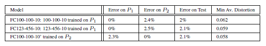
After generating adversarial examples with 100% error rates and minimal distortion for the test set, we feed them on to the training set. The results of the experiments are given below.

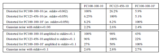
The intriguing conclusion is that adversarial data are even difficult for model trained on disjoint dataset. But the model is considerably better than others.

Conclusion

Thus, in this paper, we have demonstrated that the deep neural networks have both counter - intuitive properties - semantic meaning of individual units and their discontinuities. We also found that data with adversarial negatives in it produces very low probability. The reason could be that their chances of occurrance is relatively small. Thus the model may not be able to generalize to such data. But, a deeper research is required to understand the real working behaviour for this.

Learn more

1. Intriguing properties of neural networks (ArXiv)

Some statistics about the paper:

• Citations: 3800+ (as of 2020)
• Published at: International Conference on Learning Representations (ICLR)
• Publication year: 2014

Authors:

• Christian Szegedy (Google)
• Wojciech Zaremba (New York University)
• Ilya Sutskever (Google)
• Joan Bruna (New York University)
• Dumitru Erhan (Google)
• Ian Goodfellow (University of Montreal)
• Rob Fergus (New York University, Facebook)

Further reading:

• Convolutional Neural Networks (CNN) by Piyush Mishra and Junaid N Z (OpenGenus)