Linear Discriminant Analysis (LDA)

In order to motivate our study, we begin with a simple example. Suppose that we are statistical consultants hired by a reputable bank who are interested in predicting whether an individual will default on his or her credit card payment, on the basis of annual income and monthly credit card balance.In other words our goal is to develop a model that can be used to correctly classify the default status of a person based on his or her banking account details.

Some Notations -

In this setting, the banking account details are input variables while the default status is the output variable. The input variables are usually denoted by X and we use a subscript to distinguish between them. So X₁ may be annual income and X₂ the credit card balance, we will address input variables as predictors. The output variable in this case is default status and is often called response or dependent variable, and is typically denoted by Y. The response variable Y may be quantitative or qualitative depending on the problem that we are trying to solve. For example, height is quantitative variable and in our case the default status is a qualitative variable.

The process of predicting a qualitative variable based on input variables/predictors is known as classification and Linear Discriminant Analysis(LDA) is one of the (Machine Learning) techniques, or classifiers, that one might use to solve this problem. Other examples of widely-used classifiers include logistic regression and K-nearest neighbors.

For further studies we will assume that response variable takes on K classes (K = 2 for the example of credit card payment default, Y takes either yes or no) and the number of predictors used to make predictions about the response variable be p (p = 2 for example given before).

Mathematical Analysis of LDA being used for classification

Often the methods used for classification first predict the probability of each of the categories of the qualitative variable, as the basis of making classifications and LDA is no exception to this rule.
In LDA we model the distributions of predictors X separately for each response class, and then use Bayes' theorem to flip these around into estimates for P(Y=k|X=x) (read as probability of Y = k given X = x).
Let π_k be the probability of randomly selecting an observation that beflongs to the k^th class also known as prior probability. f_k(X) ≡ P(X=x|Y=y) denote the density function that an observation X=x comes from class k. Now we can apply Bayes' theorem to evalueate the probability of Y=k given X = x, i.e.

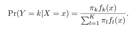
We can write P(Y=k|X =x) as p_k(X) this is also known as the posterior probability.

LDA with single predictor -

Now let us analyse the case when number of predictors is one i.e. p = 1.
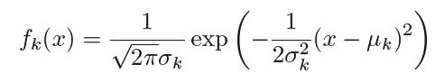
In order to get the value of above conditional probability we need to assume the probability distribution of density function f_k(X). Generally gaussian/normal distribution with with mean of class k equal to μ_k and with variance for class k as σ_k , ∴ the density function takes the form -

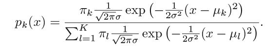
Let us further assume that all the classes have same variance σ, ∴ the posterior probability takes the form -

Hence any observation X=x is assigned to the class k for which p_k(x) is maximum on further simplifying p_k(x) we see that the observation is assigned to the class k for which

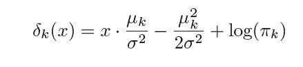
is maximum. δ_k(x) is known as the discriminant function and it is linear in x hence we get the name Linear Discriminant Analysis.
In practice, parameters μ_k, σ and π_k are not available to us in advance so they are estimated from the available dataset as follows -

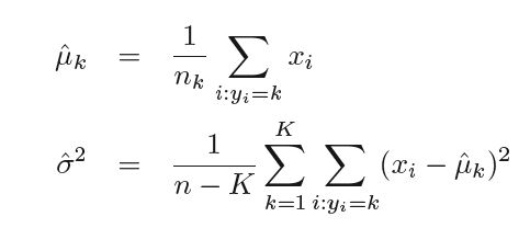
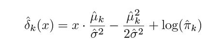
where n is the total number of observations in the training set, n_k is the number of observation in the k^th class so π_k can be estimated as n_k ⁄ n. Plugging in these estimates. we get the new estimated discriminant function as -

Summarizing

LDA assumes that distribution of the observation coming from a specific class is gaussian, estimates the values of the parameters μ_k, σ and π_k using the training data and then uses bayes' theorem to estimate the probabilities of the class to which a specific observation belongs.

LDA with more than one predictor -

We can proceed in similar way for when number of predictors(p) is greater than one. Here we get the discriminant function as follows -

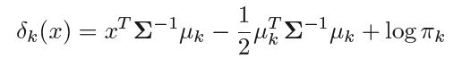
Where we assume that the observations of k^th class are drawn from Gaussian Distribution N(μ_k, Σ), μ_k is the class specific mean vector and Σ is the variance-covariance matrix common for all classes.

The inner workings of LDA for dimensionality reduction

It is often the case that we use LDA more commonly for dimensionality reduction of the dataset at hand before later classification task. We will now look how the dimensionality reduction is achieved -

1. Standardize the p-dimensional dataset (as before, p is the number of predictors).
2. For each class k, compute μ_k, the p-dimensional mean vector.
3. Construct the between-class scatter matri. S_B , and within class scatter matrix, S_W as follows - $$\displaystyle S_W = \sum_{k=1}^K S_k$$ where S_k are individual scatter matrices for each of the class k $$\displaystyle S_k = \sum_{x:y_i=k}(x - \mu_k)(x-\mu_k)^T$$ under the assumption that the class labels are uniformly distributed and $$\displaystyle S_B = \sum_{k=1}^K n_k(\mu_k - \mu)(\mu_k - \mu)^T$$ where μ is the overall mean from observations from all the K classes.
4. Next we perform the eigendecomposition of the matrix, S_W^-1S_B and the resulting eigenvalues in descending order.
   In LDA, the number of linear discriminants(eigenvectors) are at most K-1
5. Next we stack the desired number of discriminative eigenvector columns one after the other horizontally to to create a transformation matrix, W , and transform the dataset to a lower dimensional subspace by - $$\displaystyle X' = XW $$ where X' is the transformed dataset.

LDA has O(Npt + t^3>) time complexity and requires O(Np + Nt + pt) space complexity, where N is the total number of observations and p is the number of predictors and t = min(N,p), detailed analysis can be found in this paper by Cai, He and Han

Classification of Wine Recognition data using LDA in sklearn library of Python

Now we look at how LDA can be used for dimensionality reduction and hence classification by taking the example of wine dataset which contains p = 13 predictors and has overall K = 3 classes of wine.
This dataset is the result of a chemical analysis of wines grown in the same region in Italy but derived from three different cultivars. The analysis determined the quantities of 13 constituents found in each of the three types of wines. The original data source may be found here.

First we import data and standardize the dataset

import pandas as pd 
import numpy as np
import matplotlib.pyplot as plt
%matplotlib inline
df_wine = pd.read_csv('https://archive.ics.uci.edu/ml/machine-learning-databases/wine/wine.data',header = None)
df_wine.columns = ['Class label', 'Alcohol',
 'Malic acid', 'Ash',
 'Alcalinity of ash', 'Magnesium',
 'Total phenols', 'Flavanoids',
 'Nonflavanoid phenols',
 'Proanthocyanins',
 'Color intensity', 'Hue',
 'OD280/OD315 of diluted wines',
 'Proline']
 from sklearn.model_selection import train_test_split
X, y = df_wine.iloc[:,1:].values, df_wine.iloc[:,0].values
X_train, X_test, y_train, y_test = train_test_split(X,y,test_size = 0.3 , stratify = y, random_state = 0)
from sklearn.preprocessing import StandardScaler
std = StandardScaler()
X_train_std, X_test_std = std.fit_transform(X_train), std.fit_transform(X_test)

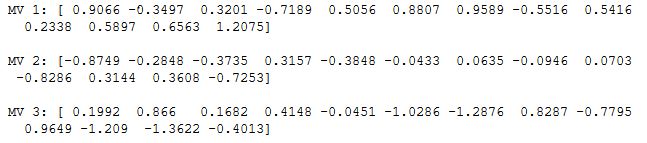
Next we calculate the mean vector for each class

np.set_printoptions(precision  = 4)
mean_vec = []
for label in range(1,4):
    mean_vec.append(np.mean(X_train_std[y_train == label], axis = 0))
    print('MV %s: %s\n' %(label, mean_vec[label-1]))

We go on to calculate within-class and between-class scatter matrix -

d = 13 # number of feature
S_w = np.zeros((d,d))
for label, mv in zip(range(1,4), mean_vec):
    class_scatter = np.zeros((d,d))
    for row in X_train_std[y_train == label]:
        row, mv = row.reshape(d,1), mv.reshape(d,1)
        class_scatter += (row - mv).dot((row - mv).T)
    S_w+=class_scatter
mean_overall = np.mean(X_train_std, axis = 0)
d = 13
S_b = np.zeros((d,d))
for i, m_v in enumerate(mean_vec):
    n = X_train_std[y_train == i+1].shape[1]
    m_v = m_v.reshape(d,1)
    mean_overall = mean_overall.reshape(d,1)
    S_b+= n*(m_v - mean_overall).dot((m_v - mean_overall).T)
print("Whithin Class scatter matrix - %sx%s" %(S_b.shape[0], S_b.shape[1]))

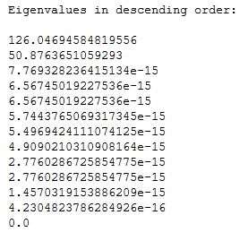
Now we proceed to calculate the eigenpairs of S_W^-1S_B

eVal, eVec = np.linalg.eig(np.linalg.inv(S_w).dot(S_b))
ePairs = [(np.abs(eVal[i]), eVec[:,i]) for i in range(len(eVal))] 
ePairs.sort(key = lambda k:k[0], reverse = True) # sorting the tuples in decreasing order of e-vals
print('Eigenvalues in descending order:\n')
for eV in ePairs:
    print(eV[0])

Now we plot the explained variance of the linear discriminants (eigenvectors) obtained -

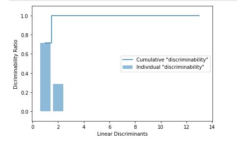
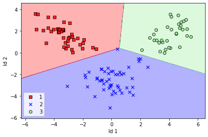
We take the first two linear discriminants and buid our trnsformation matrix W and project the dataset onto new 2D subspace, after visualization we can easily see that all the three classes are linearly separable -

With this article at OpenGenus, you must have a complete idea of Linear Discriminant Analysis (LDA). Enjoy.