This article tries to explain the advanced techniques proposed by Jason Yosinskiet al. to understand the hidden working pattern of Neural Networks in the paper "Understanding Neural Networks Through Deep Visualization". I personally like this paper very much because it is simultaneously both advanced and explains those concepts in a easier way. Now let us explore through the paper.

Introduction

The last few years have seen tremendous changes in the advancement of deep neural networks. This is particularly true in case of convolutional neural networks. Thanks to improved computational power (such as GPUs), better training techniques (such as dropouts), better activation units (such as rectified linear units), advanced larger labeled datasets for making all these happen.

Despite of these advancements in deep neural networks, we are still not able to completely understand the working of these networks. For example, AlexNet has over 60 million learned parameters. Understanding them helps us to understand their working and make further improvements. Their working still remains a black box. Understanding their intuitive properties help us develop advanced features. For example, the deconvolutional technique used to study the hidden features helps us to make a small architectural change in the convolutional filters which paved way for the development of state of art performance of ImageNet in 2013. In addition to researchers, these finding would also benefit those who are new to deep learning and mostly use predesigned packages.In order to serve these purposes, we have developed two tools.

The first tool is a software that continuously plots the activation functions of the each layer of a deep neural network for user provided images and videos. The second tool helps us to visualize the features learnt by each perceptron at every layer which helps us take better decisions and adjustments.

One approach is to study each layer as a whole because each neuron interacts with each other in a layer. Thus, this approach is used to identify each neuron's contribution to the complete DNN. Another approach is to represent the function computed bye each neuron. This can be performed in two different methods - dataset centric and network centric. The dataset centric approach requires both a trained network and a streamline of data whereas the network centric approach requires only a trained network. Dataset centric approach displays images which had high or low activation function. Network centric approach on the other hand obtains these images directly from the trained network.

These gradient based approaches are very simple to understand and apply. But while optimizing them, they tend to produce images which are in no way similar to natural images. These are caused due to collection of hacks. They cause high or low activation function, extreme pixel values and structured high frequency patterns. But information about these hacks need not be understood through these gradient approaches. They can be explained by the linear behavior of neural networks. If we are able to regularize them accordingly, we can utilize them properly. Thus, we developed three additional forms of regularization which ultimately produces more recognizable, optimization based images.

Visualizing Live Convnet Activations

Our first method involves plotting each neuron of each layer against the input images or videos. In case of neural networks, the order of firing of neuron is completely random and does not have an pattern. However, in case of a convolutional neural network, we mostly use 2D images. Thus, applying filter in the form of 2D convolutions help us obtain respective activations and along the two spatial dimensions.

This plot for conv5 layer with size 256 x 13 x13 is shown below. It consists of 256 grayscale images of size 16 x 16. The images are tiled together into a 16 x 16 grid in row major order. Since the layer size is small and the only one layer is used, all the information can be contained in the screen below along with the intuitions obtained.

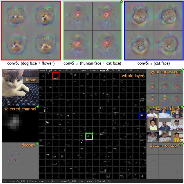
1. We find that the results are completely local. In other words, they capture entities such as flowers, fruits, faces etc.
2. When the images are streamed from google images, they give high confident scores. On the other hand, when the data is streamed from webcams, they provided incorrect classification with low probability. This is mainly due to lack of those classes in the training dataset.
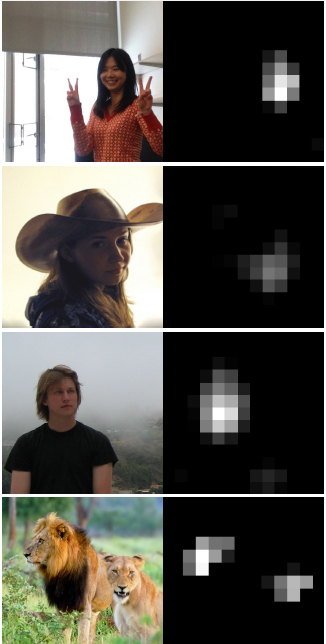
3. The lower layers computations are most robust compared to last three sensitive layers. Though images of face are not present in the 1000 class training set, they can be able to detect human and lion faces due to partial recognition as shown below.

Visualizing via Regularized Optimization

Another methodology is introducing multiple regularization methods to the bias images found during the optimization phase to more visually interpretable images. Let us consider an image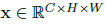
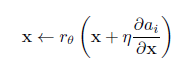
where C represents 3 different color channels, W represents width and H represents height. When this image pass through a neural network, it causes an activation along with many regularizations. In order to perform the regularization, we map an operator to the images directly. This method is very simple and easy to implement within a gradient descent as they can take small regularized baby steps towards the required direction. A single step in gradient descent is represented as shown below.

We have explored four different regularizations each to overcome specific difficulties.

L2 Decay

This method tries to prevent the domination of small number of large values. These values are outliers and are not at all useful for both modeling and data visualization. This can be implemented as follows.

Gaussian Blur

Producing images through gradient ascent produces high frequency information leading to high activation which are neither realistic nor interpretable. Using gaussian blur, we can penalize this high frequency information. Convolving (mathematically multiplying with a matrix) with a blur kernel in each step is computationally expensive. Thus, we add another hyperparameter to make sure convolving happens only after several optimizations. Multiplying once with a large kernel is similar and has same effect as multiplying many times with small kernels. Thus, this method decreases the computational costs and its implementation is represented as shown below.

Clipping pixels with small norm

The above two regularization methods are for dealing with high amplitude and high frequency information respectively. Now, the left out x* which has small and smooth information has to be dealt with. Since we have applied gradient ascent with respect to other pixels in x*, all the entries will be non-zero small values and tend to show some pattern. Thus, it gives equal importance to both required information and the non essential ones. By using this regularization, we compute the norm for each pixel and set those with very small values to zero. Thus, it highlights only the required information.

Clipping pixels with small contributions

Instead of nullifying the small pixel values, we can calculate their contributions and clip those with small contributions. The contribution can be calculated as |a(X)-a(X_j)| where X_j is x with its jth pixel set to zero. Though this process is computationally slow, linearizing them highly improves the speed of the model. Clipping all the values to zero would lead to higher activation function. Thus we only clip those which are not useful to define the required feature as defined by the gradient ascent.

Combined effect

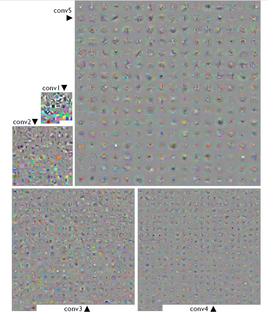
These individual parameters have good effect on producing interpretable images. Their effects are shown in the below image.

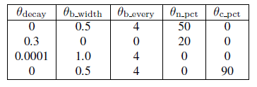
However, their combined effect shows huge influence. But we have to determine the hyperparameter for each of these regularization methods. Thus we run a random hyperparameter tuning on 300 possible combinations on the ImageNet dataset. Then, we have finalized four of those parameters combinations which has shown better performance. They are tabulated below.

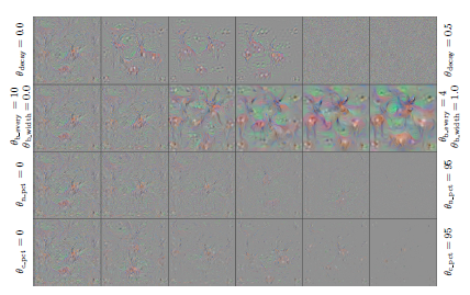
The results thus obtained for the "gorilla" class is shown in the image below.

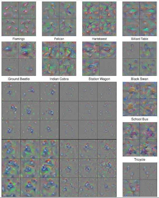
Some of them have small frequency, some have high frequency, some have sparse detailing and some have dense detailing. We found that the set of hyperparameters on the lower left corner to be the best as they perform better than the others. But more intuition can be obtained if all of them are shown together. The optimization results obtained for the all the selected units on all layers are shown in the below image.

Why are gradient optimized images dominated by high frequencies?

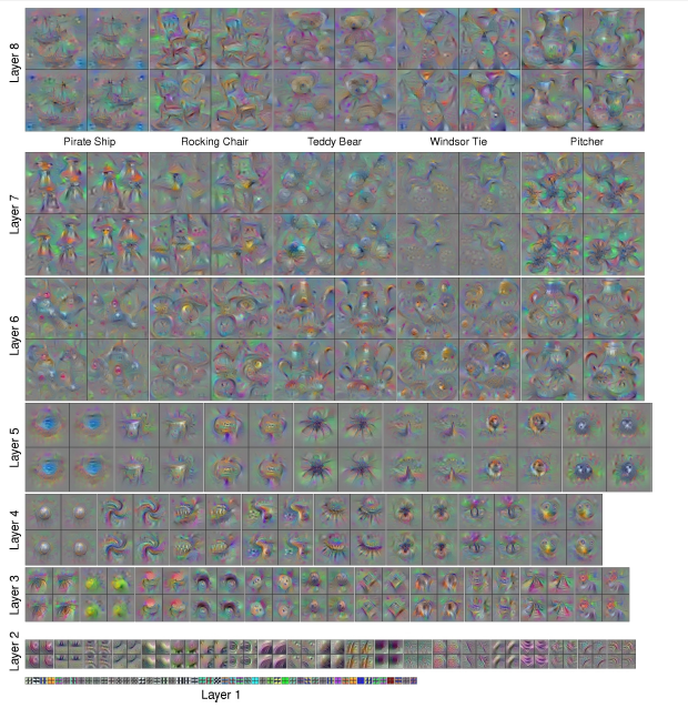
When the images were produced by gradient ascent to maximize the activation, this tend to produce high frequency information. This is because the edge detectors detect the edges in a particular layer during gradients. They are then passed to next layer during back propagation. This is the only hypothesis possible to explain this behavior. However more study has to be done to conclude this proposition. The edges or features captured by various layers of the network are shown below.

Discussion and Conclusion

The study by first tool reveals that the representational channels correspond to specific natural images while not all of these channels correspond to them but some are distributed. Thus, further research is required to understand whether they are local to a single channel or distributed across various channels.

The second tool - new regularization methods that enable improved, interpretable, optimized representations of DNN models to help researchers understand their network better and improvise it. Discriminative networks which are application specific tend to be easily fooled. For example, a discriminate model to detect jaguar identifies its spots on thee fur whereas a non discriminative model tend to capture its four legs. Thus, it is very difficult to obtain an image from a large distribution of images and then transforming it iteratively to obtain a recognizable image which satisfy both prior and posterior for any specific class.

But by using the hyperparameters obtained through our model, we are able to obtain these generative images through discriminately learned prior from the distribution of data. Now, it is possible to spot the jaguar's spots along with its legs to generate images which are realistic in nature.

Learn more

1. Paper "Understanding Neural Networks Through Deep Visualization" on ArXiv (PDF): this
2. Deep Neural Networks are Easily Fooled: High Confidence Predictions for Unrecognizable Images by Murugesh Manthiramoorthi at OpenGenus
3. One Pixel Attack for Fooling Deep Neural Networks by Murugesh Manthiramoorthi at OpenGenus
4. Machine Learning topics at OpenGenus