
Open-Source Internship opportunity by OpenGenus for programmers. Apply now.
Reading time: 15 minutes
Sammon mapping (also known as Sammon projection) is an algorithm that maps a high dimensional data to lower dimensional data by preserving the structure of inter point distances in the original data.
It was developed by John Sammon in 1969.
Introduction: Dimensionality Reduction and Principal Component Analysis
It is often necessary to reduce the dimensionality of a dataset, in order to improve our analysis, or to facilitate visualization. For the purposes of computer vision, we are most often interested in reducing the dimensionality of a large set of real-valued vectors (representing points in some high-dimensional space), and in the course of such reduction, it is useful to preserve structure as much as possible — that is, the geometric relations between the original data points should be left intact to the greatest extent feasible. A very important task is Dimensionality Reduction. This can be done via PCA (Principal Component Analysis). This is nothing but analyzing the various variables of the data and finding out the contribution of each variable towards the calculation of the output and finding out two variables which contribute the most to the output. While PCA simply maximizes variance, we now want instead to maximize some other measure, that represents the degree to which complex structure is preserved by the transformation. Various such measures exist, and one of these defines the so-called Sammon Mapping, named after John Sammon, Jr, who initially proposed it.
Multidimensional Scaling
PCA has a drawback. If all the data variables have different variances then the contribution of each of these variables towards the output will be much lesser. Hence, scaling is required to bring all the variables to a similar variance, between 0 and 1. And then the contribution to all variables can be calculated.
Sammon Mapping
Unlike traditional linear dimensionality reduction techniques (such as PCA), the Sammon mapping does not explicitly represent the transformation function.Instead, it simply provides a measure of how well the result of a transformation(i.e. some lower-dimensional dataset having the same number of points as the original) reflects the structure present in the original dataset, in the sense described above. In other words, we are attempting not to find an optimal mapping to apply to the original data, but rather to construct a new lower-dimensional dataset, which has structure as similar to the first dataset as possible.
Math Behind Sammon Mapping
We will represent the original dataset as N vectors in L-dimensional space, given by Xi, i = 1, . . . ,N. We seek to map these into d-dimensional space (with d < L), to give vectors Yi, i = 1, . . . ,N. For simplicity, write dij for the pairwise distance between Yi and Yj , and similarly dij for the distance between Xi and Xj (Sammon assumes the metric here to be Euclidean, though this is not strictly necessary).The amount of structure present in the original but lost in the transformed dataset is then measured by an error E, defined as:
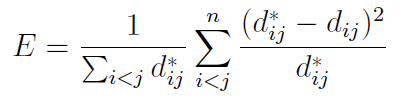
Essentially, the error is given by summing up the squared differences (before versus after transformation) in pairwise distances between points; the summations are over the range i < j so that each pairwise distance is counted once (and not a second time with i and j swapped). The tendency to preserve topology (mentioned above) is due to the factor of dij in the denominator of the main summation, ensuring that if the original distance between two points is small, then the weighting given to their squared difference is greater.
Implementation
The error E provides us with a measure of the quality of any given transformed dataset. However, we still need to determine the optimal such dataset, in terms of minimizing E. Strictly speaking, this is an implementation detail and the Sammon mapping itself is simply defined as the optimal transformation; Sammon describes one method for performing the optimization. The transformed dataset Yi is first initialised by performing PCA on the original data (an arbitrary, random initialisation is sufficient, but using the principal components improves performance somewhat — see below). Then, we repeatedly update the Yi using steepest descent, considering the gradient of E with respect to the Yi, until satisfactory convergence is achieved. This optimisation problem has rather high dimensionality (proportional to the number of data points), and hence other more modern techniques, such as simulated annealing, could beneficially be applied in order to achieve
better convergence properties and avoid local minima.
PCA vs Sammon Mapping
The original dataset contains three mutually perpendicular circles in six dimensional space, meeting at a point. Now we find out the PCA and Sammon mapping projections.
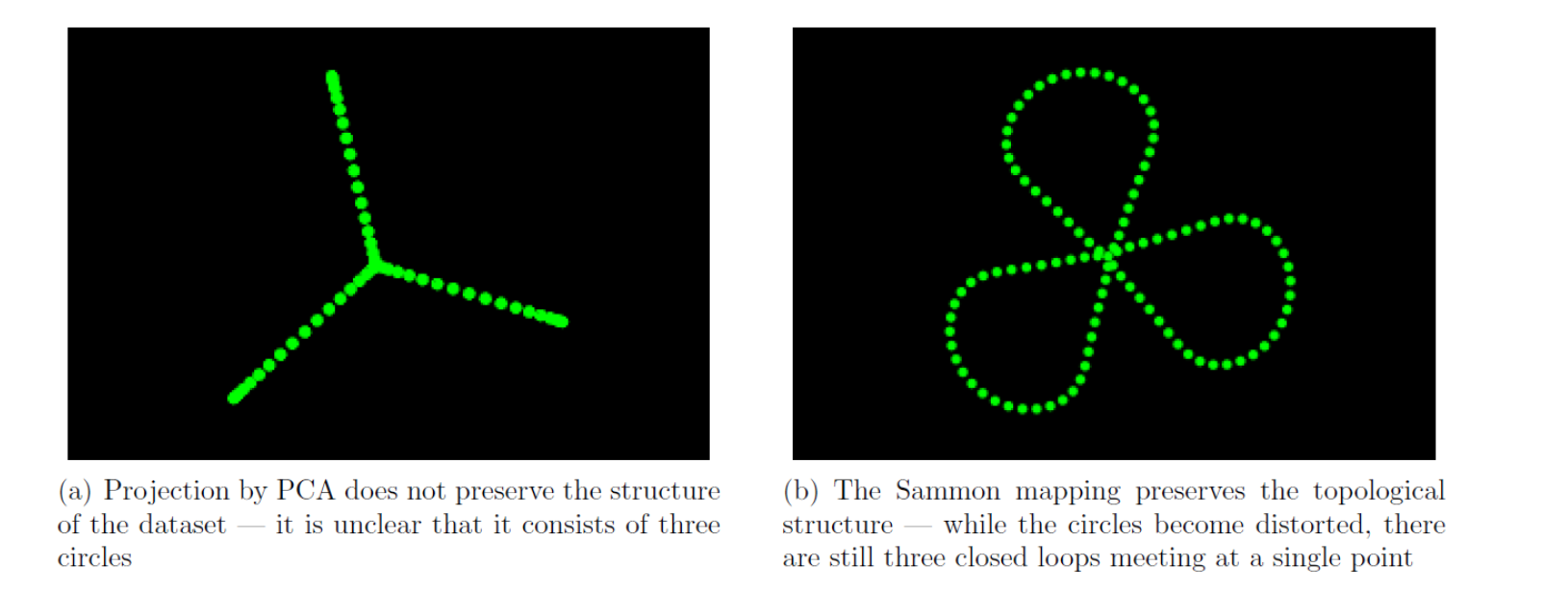
Figure illustrates how the mapping can reduce a six-dimensional dataset to a two dimensional one, while preserving the topological structure. Hence it is very clear that Sammon mapping is the better alternative.