Range Searching is one of the most important fields in Computational Geometry and have applications in database searching and geographical databases. We have explored Algorithms & Data Structures for Range Searching (Multi-dimensional data). This article at OpenGenus gives an Advanced knowledge in this domain.

The problem statement goes as follows:

Given a set S of n points in a plane in a d-dimension we are allowed to build an appropriate data structure that supports query of the following kind:

For some range (let's call it delta) we should return two kinds of query:

1. reporting query return all points in delta intersection S
2. the cardinality of the query set, i.e the number of points in mod(delta intersection S)

Range is a predefined family of subsets.

For example consider the points in the plane, we are given the delta which is nothing but the range and are required to return either of the two queries. This can be illustrated in the figure below

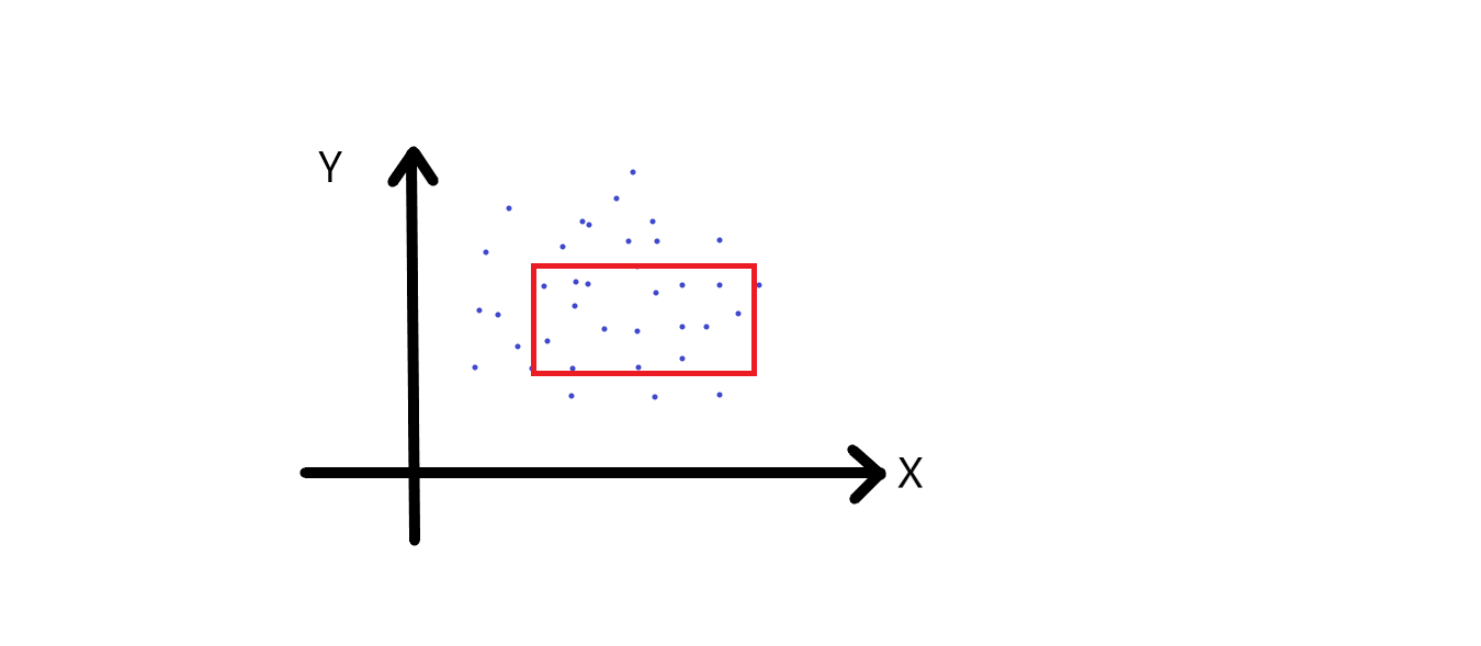
In the above image the range takes the shape of a rectangle. Note that range can be of any shape like spherical, triangle etc. This is just a 2-dimensional range searching. Also, this is a common query in database searching. For a complete beginner in databases, consider this, we are given a table holding information of various students enrolled in a particular course. And the columns are his id(which is unique), age, address, contact etc. In a database (a database can be defined as structured set of data, like this one), if someone needs to find all the students who are from section 'B' , then they will perform a search on the database to obtain the result.

You might be thinking where does this fit with the information given in the beginning. So, we are searching the entire database with one specific attribute (section), so a single attribute defines a single dimensional range searching. We are calling it single because we are only searching the section column. In the same way, the number of attributes become the number of dimensions where the searching is performed. The above example was a simple one, in real world, when the data has to be searched a number of attributes are applied to get a more specific result.

In the above diagram query range is Cartesian Product (the multiplication of two sets to form the set of all ordered pairs) of two intervals. So, if you want all the points that have coordinates between x1, x2 and y1 and y2, then we have the we have Cartesian product of two one dimensional intervals.

Now, we need to build data structure that would support these queries. This of course is on the assumption that there are a series of queries that are being asked.

General Time Complexity

In a very trivial case of points on a line, the time complexity for the first query is O(n) or size of the output. This isn't really ideal and what we come across more often here is a polylogarithmic complexity or some polylog plus size of the output. So, this is basically objective when we build a data structure and also almost equally important what other parameter is which is the size of data structure and somewhat less important is the preprocessing time.

We can start with a one-dimensional model and build it up to higher dimensions.

One-dimensional range searching

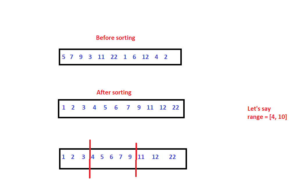
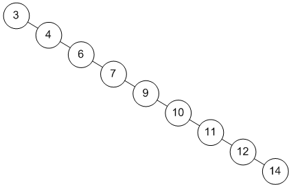
This is probably the easiest one. We are given some set of points S of size n, and a closed interval describing the range, we have to return all the points that belong to the range. We need to report all points between, let's say x1 and x2.
We start this by preprocessing. We need to locate the starting point of the range or the left boundary using binary search and start traversing, and return the values. This process can be illustrated in the figure below.

Time Complexity
O(logn) for binary search and O(n logn) for sorting.

This was fine, but what if we had to insert or delete values prior to the reporting query. This is a very natural modification.

1. The data structure we can use here is a balanced binary search trees. That would input the set of points, and for any modification, we simply have to delete the current value and insert the new value.
2. We can use self-balancing trees for this purpose such as AVL trees or Red-Black trees.

Binary Tree is a tree, which in turn is a hierarchical data structure where each node can be defined with a value of any data type and two pointers that point or store address of the next elements in the hierarchy. The pointers are also called as children, with them being left and right child; the root node is referred to as parent. And a binary tree has a maximum of two children.

Binary Search Trees is a binary tree which has the following properties:

1. The left subtree's data must be less than that of the root.
2. The right subtree's data must be greater than that of the root.
3. These two properties must be followed by the entire tree , i,e the left and the right subtrees must also be BSTs.

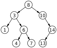
The above figure illustrates a BST, where the values of the left child is less than the node value and the value of the right child is greater than the node value.

For the given set of points we can insert them into a self balancing BST

1. Generally, the BST will perform operations such as searching, insertion and deletion in O(log n).
2. But, the problem with using a regular BST is that the order of tree, which is the order in which the insertion has done decides the shape of the tree. This leads to the worst complexity of O(n) for all the above mentioned operations. Consider this example

Consider a list that is sorted, and when we try creating a BST for these elements, we get the above tree. Since every element is greater than or equal to the current element, the insertion is done on the right. The tree is skewed towards the right, hence the name right skewed BST Any operation on this tree will give the worst time complexity.
3) Now that we've discussed skewed trees, we'd also like to define balance factor. It can be defined the difference between height of left subtree and the right subtree.
4) In ideal cases, this should be -1, 1 or 0.
5) Therefore we will switch to self balancing trees such as AVL trees, Red Black trees etc.

Self-Balancing Binary Search Tree

As the name suggests they are BSTs that balance themselves, which means that they undergo some operations in order to maintain the ideal balance factor, which as discussed above should be -1, 1 or 0 to get the ideal time complexity of O(log n).

How do Self-Balancing-Tree maintain height?
A typical or we can say a crucial operation done by trees is rotation. If insertion of a value leads to imbalance in the balance factor, the tree adjusts its height in order to retain the ideal balance factor. This is called rotation. There are many self-balancing trees like Red Black trees, AVL trees and so on. In this case, we opt for Red Black trees as they insert in constant time, with all other time complexities being almost same for Red Black and AVL trees.

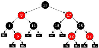
Red-Black Tree is a self-balancing Binary Search Tree (BST) where each node is required to follow certain rules such as

1. The color of the node has to be either red or black
2. The root of tree is always black.
3. There are no two adjacent red nodes (A red node cannot have a red parent or red child).
4. Every path from a node (including root) to any of its descendant NULL node has the same number of black nodes.

Range Searching in self balancing BST
Let's call the range [x,y]. Compare the root node with x and y.

1. if root value is greater than x and y, we have to search in the left subtree and return values.
2. if root value is lesser than x and y, we search in the right subtree and return values. These two cases are called total overlap.
3. there's something called partial overlap where x belongs to left and y belongs to right. In that case we have to search both the subtrees.

Time Complexity
We can say that O(q*log n) will be running time. This includes constant time for insertion and O(log n) for other operations. q denotes the number of queries. This of course is valid when we are using Red Black Trees.

Higher Dimensions (2 or more)

The variations in single dimensions with respect to range was basically open or closed intervals. But, when we go to higher dimensions, two or more, the range intervals could take up any shape or form.

1. Rectangular range query, basically it was orthogonal. This was the cartesian product of the range

[x1, x2] * [y1, y2]

2. Rectangular range query need not to be orthogonal, it can be aligned as well.
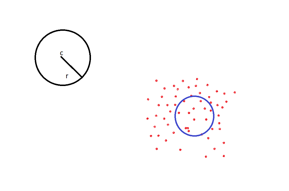
3. Circular range queries, basically a circle with radius 'r', centered as 'c'. Now what are the points inside this circle? That's basically circular range query.
   
4. There can be other arbitrary shapes, in linear boundaries, it could be a simple polygonal query
   
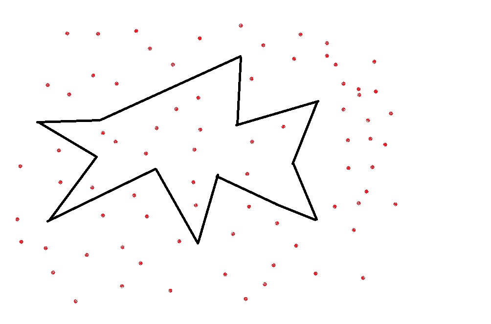
   For a polygon like this, we certainly cannot answer the query "if a point lies inside or outside the polygon" in linear time compared to the previous one-dimensional model. We can do a ray shooting algorithm .Ray shooting or Ray casting is the use of ray–surface intersection tests to solve a variety of problems in 3D computer graphics and computational geometry. This will perform the task in O(log n) time.
   We can actually break this polygon into triangles to answer the question easily.
   
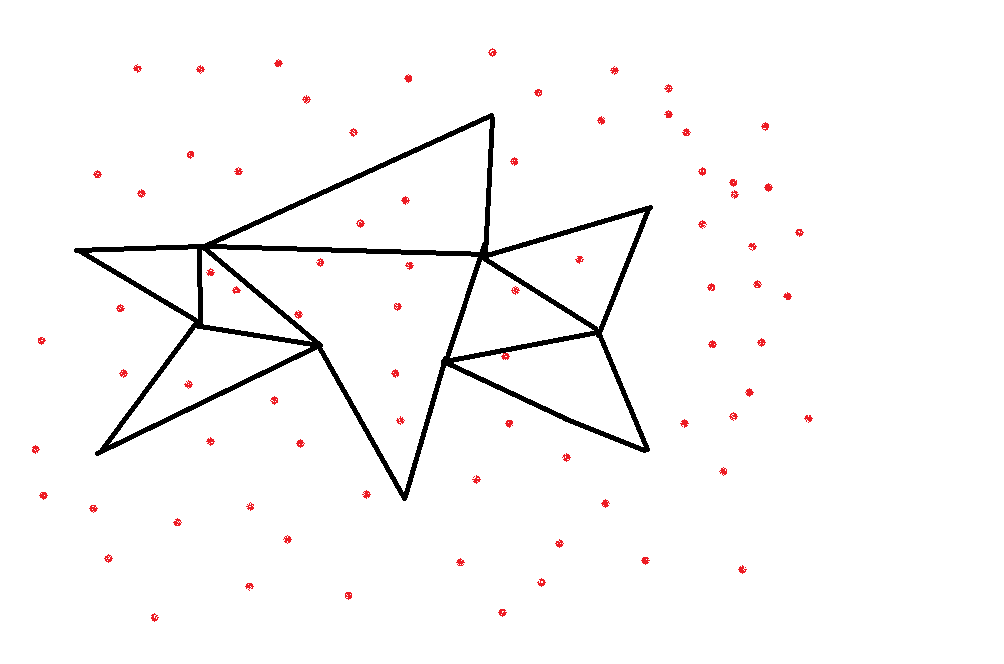
   We can perform a triangular range query on each triangle and union these answers to get the final answer. Sometimes, simple addition won't work. There is a natural generalization that uses some kind of operator to combine the answers of the triangles.
   We can combine the results of the individual triangles using semi-group operators.
   Consider an example, consider a set of points, these points have attributes such as height. Given a range we need to find the highest y-axis in this intervals.

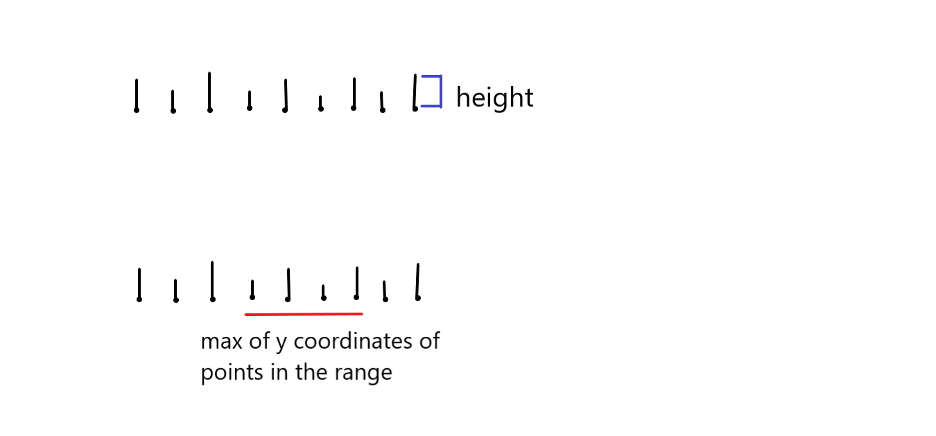
So, the first job to find out which points are we talking, which points are in consideration. After that we are going to do kind of max of the y coordinates of the points in the range. So, this max is an operator. This is not a two dimensional problem where there are two, these are the points and we need to return all the points that occur in this rectangle this poblem. These problems, they are not the same. So, this is actually a one-dimension. Range query problem where there is an underlying operator which is a max operator and semi-group, basically means associative operator. So, it is this operator will also act on the results of the range query and that is how we will get the final answer. So, this is also a range query problem, but it is a more complex range query problem and you can really sort of build very complex range query problems for more and more general definitions.

2-dimensional range searching

Consider a triangular range query, in the above part, we've seen how we can disintegrate polygon into triangles. But, for the triangles one of the approach which we can apply here is clustering
Given some point, we first cluster them into regions, clusters can be defined as points that are of close proximity. Look at the figure below.

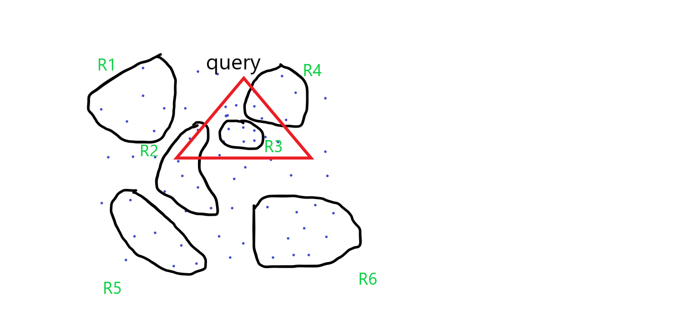
These groupings which can be defined easily. It is not a very complicated shape and which will require, have a large descriptive complexity. So, they have some simple description which can be accessed in constant time.
Our triangular query is overalapping four different regions. We can establish some facts here

1. We don't need R1, R5 and R6 as they have nothing to do with the query.
2. We take the R3 completely since it is lying inside the triangle.
3. These two are the extreme cases, for the rest, well, we know it is the intersection of R2 and R4, but we have no idea how many points are inside R4 or R2. Because we only know about the description of this region and don't know how the points are distributed inside.

We have not kept track of that and it is very difficult to. So, based on this information, we have to look further or examine how many points in R2 and R4 are contained inside the query triangle.
So, again R1 is a set of points, R2 is a set of points and we are going to again do the same thing within these regions right. So, maybe we will just have some more clusters here.

So, for the final answer it is going to be the union of the range query of this triangle with R2 and R4. So, we have branched out now.
Unfortunately, now this whole thing, this entire thing the set of points as R. So, the range query R is the regions that completely lie inside, that is taken care of the first level itself. The regions that do not intersect, that is also taken care of, but recursively we need to handle all the regions that partially, have some partial overlap with this. So, it becomes union of R2 and R4 which actually is not good news because if you want to write any kind of recurrence relation for the query time, then from a single point, you could have two way branching and that. If you have two way branching or three way branching the whole thing may not turn out to be very efficient. In this example we have seen only two branches, there are cases where the number of branches can be significantly higher.
After all, we want our goal is to report in time proportional to a fixed logarithm term or a poly logarithmic term plus the number of output points but any kind of reference where you have so many branches is unlikely to be very efficient. So, that is why we have
to be careful when we define this partitioning.

So, this is a very general approach to range query. That given set of points we would like to partition them in a certain way and then the query will be answered as union of which partitions this query triangle or whatever the query is, the range has non-trivial intersection way, if it fully overlaps, no problem. It does not overlap at all, no problem but partial overlaps are the one which have to be recursively sort of handled.

k-d trees

In higher dimensions we prefer the range trees. It is an ordered tree data structure to hold a list of points. It allows all points within a given range to be reported efficiently, and is typically used in two or higher dimensions. We will be looking a special type of the range trees called k-d trees where the d stands for dimension.

Now that we are in two dimensions, we will look at a special way of defining this partition. So, this is very arbitrary partition. In this way, where we could have a four way, five ways. We don't know how many ways we have to recursively look forward. So, we want to
somehow bound the number of branches that we are going to have.

Let P be a set of points in a two dimension.

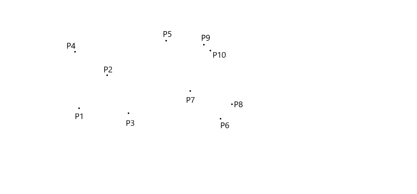
The basic assumption is no two point have same x-coordinate, and no two points have same y-coordinate. Let’s consider the following recursive definition of the binary search tree : the set of (1- dimensional) points is split into two subsets of roughly equal size, one subset contains the point smaller than or equal to splitting value, the other contains the points larger than splitting value. The splitting value is stored at the root and the two subsets are stored recursively in two subtrees.
Each point has its x-coordinate and y-coordinate. Therefore we first split on x-coordinate and then on y-coordinate, then again on x- coordinate, and so on. At the root we split the set P with vertical line l into two subsets of roughly equal size. This is done by finding the median x- coordinate of the points and drawing the vertical line through it. The splitting line is stored at the root. Pleft , the subset of points to left is stored in the left subtree, and Pright, the subset of points to right is stored in the right subtree. At the left child of the root we split the Pleft into two subsets with a horizontal line. This is done by finding the median y-coordinate if the points in Pleft . The points below or on it are stored in the left subtree, and the points above are stored in right subtree. The left child itself store the splitting line. Similarly Pright is split with a horizontal line, which are stored in the left and right subtree of the right child. At the grandchildren of the root, we split again with a vertical line. In general, we split with a vertical line at nodes whose depth is even, and we split with horizontal line whose depth is odd.
The below figures illustrates this clearly.

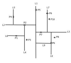
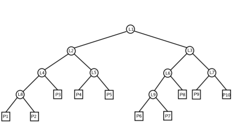
The k-d tree for the above figure will be

Algorithm

Let us consider the procedure for constructing the kd-tree. It has two parameters, a set if points and an integer. The first parameter is set for which we want to build kd-tree, initially this the set P. The second parameter is the depth of the root of the subtree that
the recursive call constructs. Initially the depth parameter is zero. The procedure returns the root of the kd-tree.
Procedure name: BUILDKDTREE(P,depth)
Input: A set of points P and the current depth depth.
Output: The root of the kd-tree storing P.

1: if P contains only one point
2: then return a leaf storing this point
3: else if depth is even
4: then split P into two subsets with a vertical line l through the median x-coordinate of the points in P.Let P1 be the set of points to the left of l or on l, and let P2 be the set of points to the right of l.
5: else split P into two subsets with a horizontal line l through the median y-coordinate of the points in P.Let P1 be the set of points to the below of l or on l, and let P2 be the set of points above l.
6: vleft←BUILDKDTREE(P1, depth +1).
7: vright←BUILDKDTREE(P2, depth +1).
8:Create a node v storing l, make vleft the left child of v, and make vright the right child of v.
9:return v.

Time Complexity
The most expensive step is to find the median. The median can be find in linear time, but linear time median finding algorithms are rather complicated. So first presort the set of points on x-coordinate and then on y-coordinate. The parameter set P is now passed to the procedure in the form of two sorted list. Given the two sorted list it is easy to find the median in linear time. Hence the building time satisfies the recurrence,

T(n)=O(1), if n=1,
O(n)+2T(ceil(n/2)),if n>1

which solves to O(q*n log n), where q denotes the number of queries. Because the kd-tree is the binary tree, and every leaf and internal node uses O(1) storage, therefore the total storage is O(n).

Other data structures that can be used for range searching

Apart from k-d trees and balanced binary that we saw, there are other data structures as well that can be used for range searching.

1) Quad Trees

Quad trees as the name suggest have either zero children or four children. They can efficiently store points in any arbitrary dimension.
For a two-dimensional area, we can build a quadtree by implementing the following steps

1. The current two-dimensional space is divided into four boxes.
2. If a box contains one or more points in it, build a child object, storing in it the two dimensional space of the box.
3. Else, do not build a child for it.
4. Perform recursion for each of the children.

The maximum running time for range searching using quadtrees is O(n+h) where n is the number of points and h being height.

2)R(Region)-trees

The R-tree can organize two (and higher) dimensional objects by representing the data by a minimum bounding rectangles (MBR). Nodes of the tree store MBRs of objects or collections of objects. And each node bounds it's children. The leaf nodes of the R-tree store the exact MBRs or bounding boxes of the individual geometric objects, along with a pointer to the storage location of the contained geometry.
All non-leaf nodes store references to several bounding boxes for each of which is a pointer to a lower level node. The tree is constructed hierarchically by grouping the leaf boxes into larger, higher level boxes which may themselves be grouped into even larger boxes at the next higher level.
The average case time complexity is O(logM n) where M is MBR and n being the number of nodes.

3)Priority R-trees

The prioritized R-tree is basically a hybrid between a k-dimensional tree and a r-tree. It defines a given object's MBR as a point in N-dimensions, which is represented by an ordered pair of the rectangles. There are four priority leaves that represent the most extreme values of each dimensions included in every branch of the tree, hence the term "prioritized".
A window query(i.e information retrieval) is done by traversing the sub-branches. However, before traversing the R-tree checks if there's any overlap in its priority nodes. The traversal of the sub-branches is done by checking whether the least value of the first dimension of the query is above the value of the sub-branches.By doing this an access to a quick indexation by the value of the first dimension of the bounding box is given.

Although efficient when compared to r-tree the time complexity is worse than r-tree.

4)K-D-B Trees

A K-D-B tree is a k-dimensional B-tree. This tree aims to deliver the search efficiency of a balanced k-d tree and the block-oriented storage of a B-tree which can ultimately help in optimizing the accesses to the external memory. The K-D-B tree organizes points in k-dimensional space which is similar to the functionality of a k-tree. This organization is useful for performing range-searching and multi-dimensional database queries.
K-D-B-trees subdivide space into two subspaces by comparing elements in a single domain.For example, consider the 2-D-B tree in which space is subdivided just like the k-d tree. This happens in the following way : using a point in one of the domains, or in this case, axes, all the values less than the current value fall in the left plane and the values greater than fall in the right plane, splitting it.
In contrast to the k-d tree, each half space that was subdivided is not its own node, but the nodes are stored as pages similar to the B-tree. Ans the tree this stores a pointer to the root page.
The running time for querying an axis-parallel range in a balanced k-d tree takes O(n^1−(1/k) +m) time, where m is the number of the reported points, and k the dimension of the k-d tree.

Applications

1. In addition to being considered in computational geometry, range searching, and orthogonal range searching in particular, has applications for range queries in databases.
2. Colored range searching is also used for and motivated by searching through categorical data. For example, determining the rows in a database of bank accounts which represent people whose age is between 25 and 40 and who have between $10000 and $20000 might be an orthogonal range reporting problem where age and money are two dimensions.