Understanding Recurrent Neural Networks with an example of assigning an emoji to a sentence

Reading time: 50 minutes | Coding time: 20 minutes

I am quite sure that, when you were searching for the results of recurrent neural networks online, you must have got auto-complete suggestions like “recurrent neural networks for …sequence data” and the like.

Well, that’s exactly recurrent neural nets in practice. This task of predicting the next word from the general context of the sentence is something a recurrent neural network can easily handle. More on this later. Let’s start with the fundamentals first.

So, we will discuss the following in this post:

• What are recurrent neural networks and why are they preferred over feed-forward networks?
• Issues with RNNs
• Long Short Term Memory(LSTM) Networks
• A use case of LSTM

So, what are recurrent neural networks?

They are yet another type of artificial neural networks, which are specifically designed to work on sequential data by recognizing patterns in such data. They have an abstract concept of sequential memory which allows them to handle data such as text, handwriting, spoken word, and even genomes.

What do we mean by sequential data?
Consider this. As you are reading this article, you are understanding each word based on the previous word you read and based on the overall context of the post. The independent words would be meaningless. They become meaningful only when they follow a particular sequence.
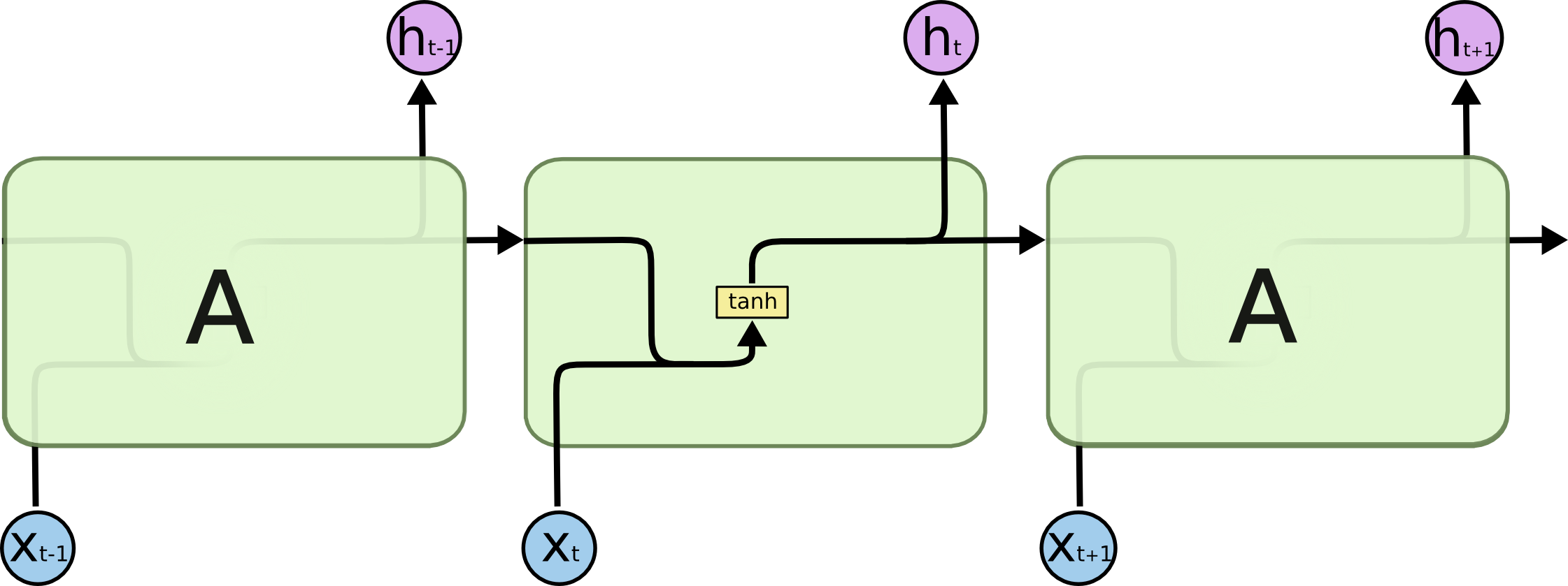
This means that we have some persistence. The same kind of persistence is shown by recurrent neural networks, owing to their structure, which is, having a loop as shown below.

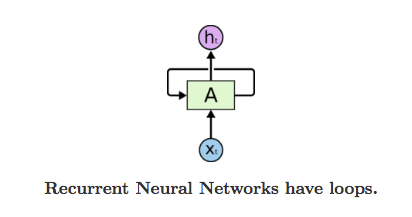
Img src: Link

In the above diagram, a chunk of neural network, A, looks at some input xt and outputs a value ht. A loop allows information to be passed from one step of the network to the next.

A recurrent neural network can be thought of as multiple copies of the same network, each passing a message to a successor. If we unroll the loop above, we will see that recurrent neural nets aren’t all that different form a normal neural net.

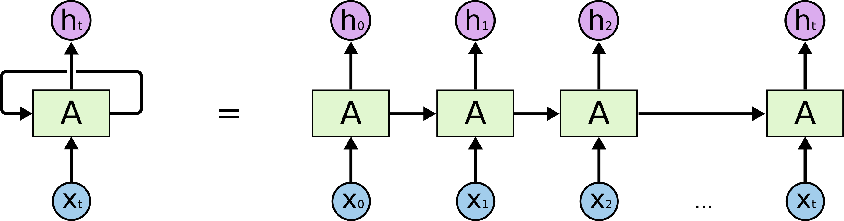
Img src: link

This chain-like nature reveals that recurrent neural networks are intimately related to sequences and lists. They’re the natural architecture of neural network to use for such data and which is why they have been successfully applied to problems like machine translation, image captioning, speech recognition, music generation and a lot more!
Okay, so the core reason why RNNs are exciting is because they allow us to operate over data, and so depending upon the length and number of sequences in the input and the output, we have a few categories in RNN.

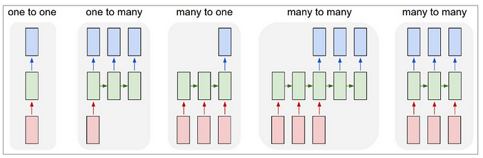
Img src: link

1. One to One: Fixed-size input to fixed-size output eg.. image classification
2. One to many: Sequence output eg.. image captioning, where the input is just an image and the output is a sequence of words
3. Many to one: Sequence input egg, sentiment classification of a text or maybe converting a text into the corresponding emoji, which is something we will be discussing in a while.
4. Sequence input and sequence output: eg.. machine translation wherein you feed a sequence of words in French and get a translated sequence in German.
5. Synced many to many: eg.. video classification, where we wish to classify each frame of the video.

Issues with RNNs

There are mainly two issues with every type of neural net(including RNN):

• Vanishing gradients or short term memory in RNN
• Exploding gradients

Vanishing gradients
As our RNN processes more steps, it has trouble retaining information from the previous steps. So, in some cases, this might not be a problem, where the word just depends on its previous neighboring word. For eg.the sentence: I can speak French very well. Now the word ‘well’ in this sentence is very intuitive to come at this place and RNN can handle such sentences effectively. But consider this sentence: I am going to France, the language spoken there is _______. Now the answer “French” here has a dependency on the word France, which is far away from it. This type of dependency is known as long term dependency, and the normal structure of RNN fails to operate over these.

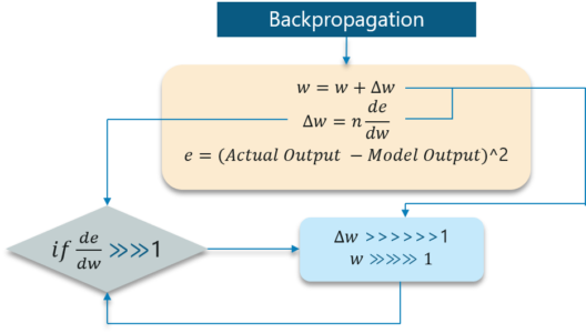
Short-Term Memory and the vanishing gradient is due to the nature of back-propagation; an algorithm used to train and optimize neural networks.
When doing back propagation, each node in a layer calculates it’s gradient with respect to the effects of the gradients, in the layer before it. So if the adjustments to the layers before it is small, then adjustments to the current layer will be even smaller.
That causes gradients to exponentially shrink as it back propagates down. The earlier layers fail to do any learning as the internal weights are barely being adjusted due to extremely small gradients. And that’s the vanishing gradient problem.

Img src: Link

Gradients shrink as they backpropagate down.

Because of vanishing gradients, the RNN doesn’t learn the long-range dependencies across time steps. That means that there is a possibility that the word “France” is not considered when trying to predict the user’s intention. The network then has to make the best guess with “there is?”. That’s pretty ambiguous and would be difficult even for a human. So not being able to learn on earlier time steps causes the network to have a short-term memory.

Exploding Gradients
The working of the exploding gradient is similar to that of vanishing gradient but the weights here change drastically instead of negligible change.

Img src: Link

Long Short Term Memory Networks

Let’s talk about LSTMs now, which are a special type of RNNs, designed to combat the issues of short term dependencies(vanishing gradients) and exploding gradients and handle long-term dependencies easily.

Remembering information for long periods of time is practically their default behavior, not something they struggle to learn!

All recurrent neural networks have the form of a chain of repeating modules of neural network. In standard RNNs, this repeating module will have a very simple structure, such as a single tanh layer.

Img src: Link

LSTMs also have this chain-like structure, but the repeating module has a different structure. Instead of having a single neural network layer, there are four, interacting in a very special way.

Img src: Link

Step by Step LSTM Walk Through
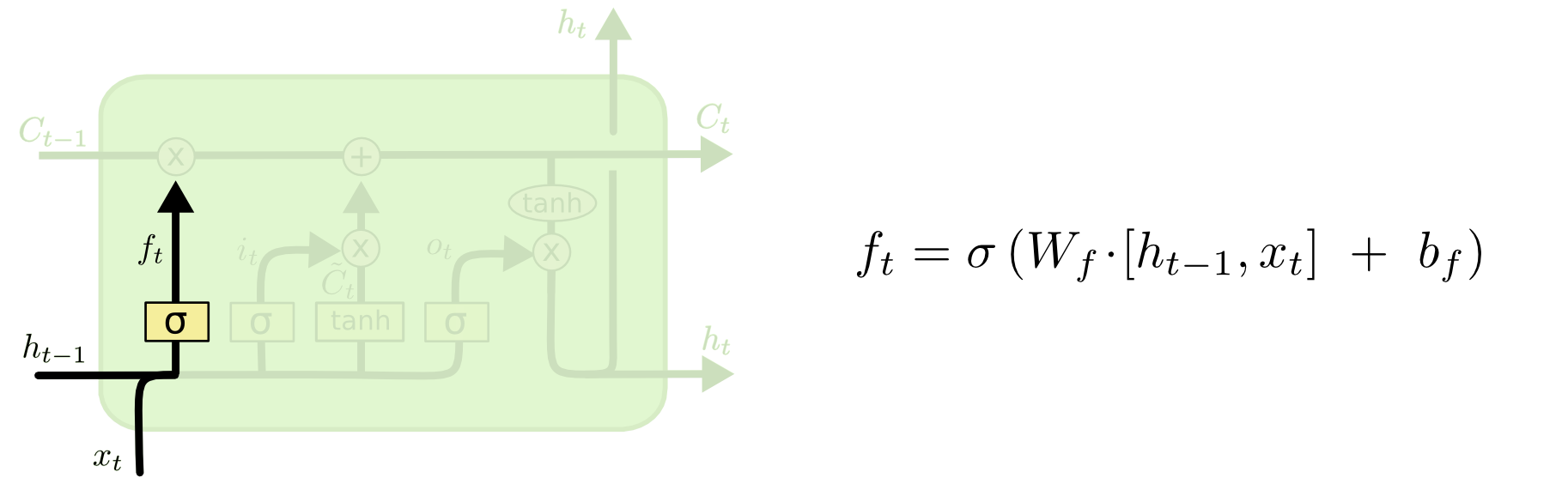
Step 1:
The first step in the LSTM is to identify that information which is not required and will be thrown away from the cell state. This decision is made by a sigmoid layer called a forget gate layer.

Img src: Link

The highlighted layer above is the sigmoid layer.

The calculation is done by considering the new input and the previous timestamp which eventually leads to the output of a number between 0 and 1 for each number in that cell state.
As a typical binary, 1 represents to keep the cell state while 0 represents to trash it.
Consider the case of gender classification, we might want to forget the old gender, whenever we see a new one. The forget layer helps the network do that.

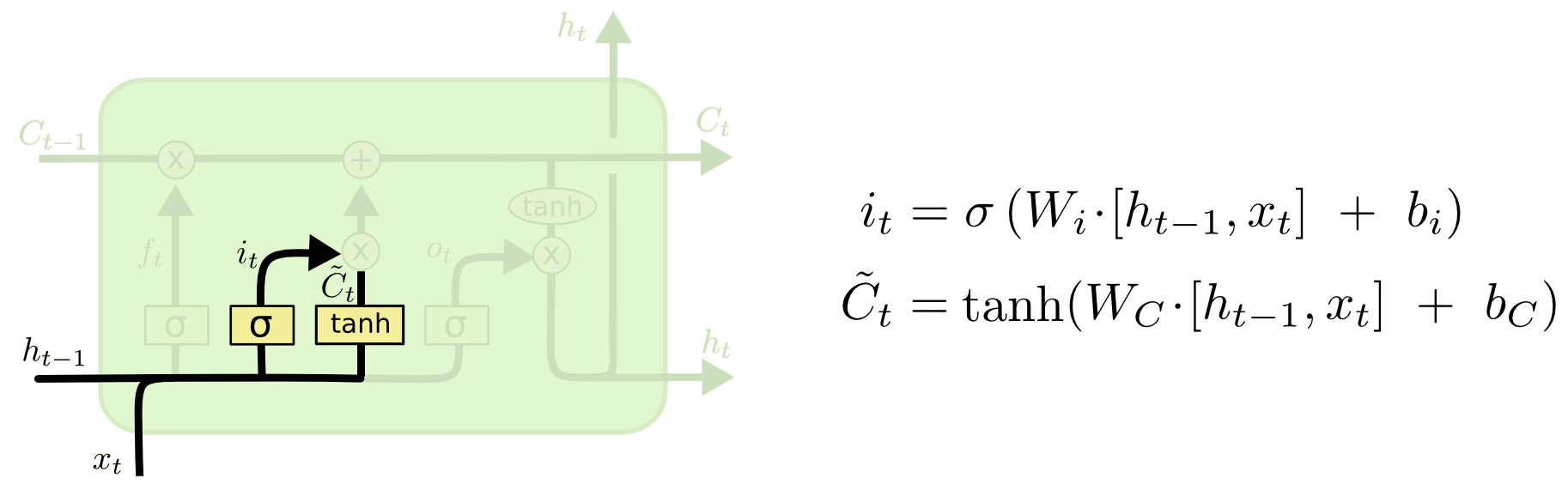
Step 2:
The next step is to decide what new information we’re going to store in the cell state. This has two parts:

• A sigmoid layer called the “input gate layer” which decides which values will be updated.
• The tanh layer creates a vector of new candidate values, that could be added to the state.

In the next step, we’ll combine these two to create an update to the state.
In the example of gender classification, we’d want to add the gender of the new subject to the cell state, to replace the old one we’re forgetting.

Img src: Link

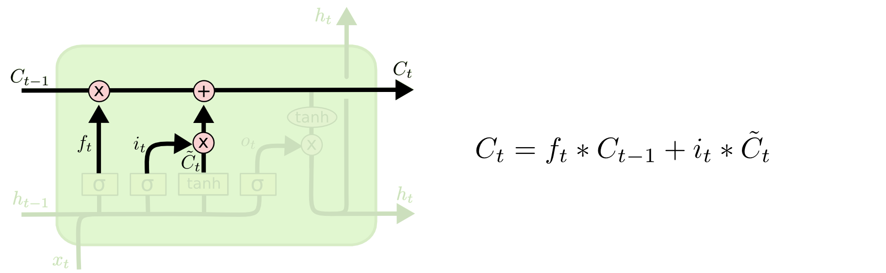
Step 3:
Now, we will update the old cell state Ct−1, into the new cell state Ct.
First, we multiply the old state (Ct−1) by f(t), forgetting the things we decided to leave behind earlier.

Img src: Link

Then, we add i_t* c˜_t. This is the new candidate values, scaled by how much we decided to update each state value.
In the second step, we decided to do make use of the data which is only required at that stage.
In the third step, we actually implement it.
In the language case example which was previously discussed, there is where the old gender would be dropped and the new gender would be considered.

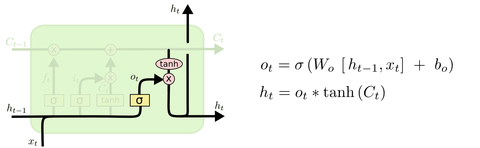
Step 4:
Finally, we need to decide what we’re going to output. This output will be based on our cell state, but will be a filtered version.

First, we run a sigmoid layer which decides what parts of the cell state we’re going to output.
Then, we put the cell state through tanh (push the values to be between −1 and 1)
Later, we multiply it by the output of the sigmoid gate, so that we only output the parts we decided to.

For the language model example, since it just saw a subject, it might want to output information relevant to a verb, in case that’s what is coming next. For example, it might output whether the subject is singular or plural, so that we know what form a verb should be conjugated into if that’s what follows next.

Img src: Link

Summing up all the 4 steps:

1. In the first step, we found out what was needed to be dropped.
2. The second step consisted of what new inputs are added to the network.
3. The third step was to combine the previously obtained inputs to generate the new cell states.
4. Lastly, we arrived at the output as per requirement.

Use Case

Okay, so as our use case , let's discuss how to assign an emoji to a sentence based on its sentiment.
This project is a part of Coursera deep learning course on Recurrent Neural Networks.
The code below is intended to demonstrate only building and working of an LSTM model and doesn’t serve the purpose of a full working project. For complete project code, head over to this notebook

1. Let's start with importing the libraries

import numpy as np
np.random.seed(0)
from keras.models import Model
from keras.layers import Dense, Input, Dropout, LSTM, Activation
from keras.layers.embeddings import Embedding
from keras.preprocessing import sequence
from keras.initializers import glorot_uniform
np.random.seed(1)
import matplotlib.pyplot as plt

%matplotlib inline

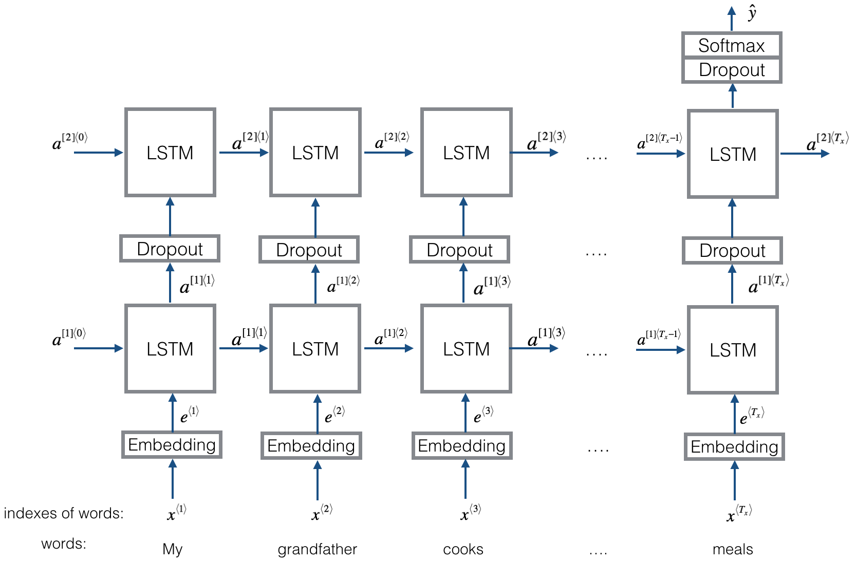
2. Overview of our LSTM model
   

3. Let's build the embedding layer now.
   In Keras, the embedding matrix is represented as a "layer", and maps positive integers (indices corresponding to words) into dense vectors of fixed size (the embedding vectors). It can be trained or initialized with a pretrained embedding. In this step, we will learn how to create an Embedding() layer in Keras, initialize it with the GloVe 50-dimensional vectors(you can find these in the notebook mentioned above).
   Because our training set is quite small, we will not update the word embeddings but will instead leave their values fixed. But in the code below, we'll see how Keras allows us to either train or leave fixed this layer.

The Embedding() layer takes an integer matrix of size (batch size, max input length) as input. This corresponds to sentences converted into lists of indices (integers), as shown in the figure below.

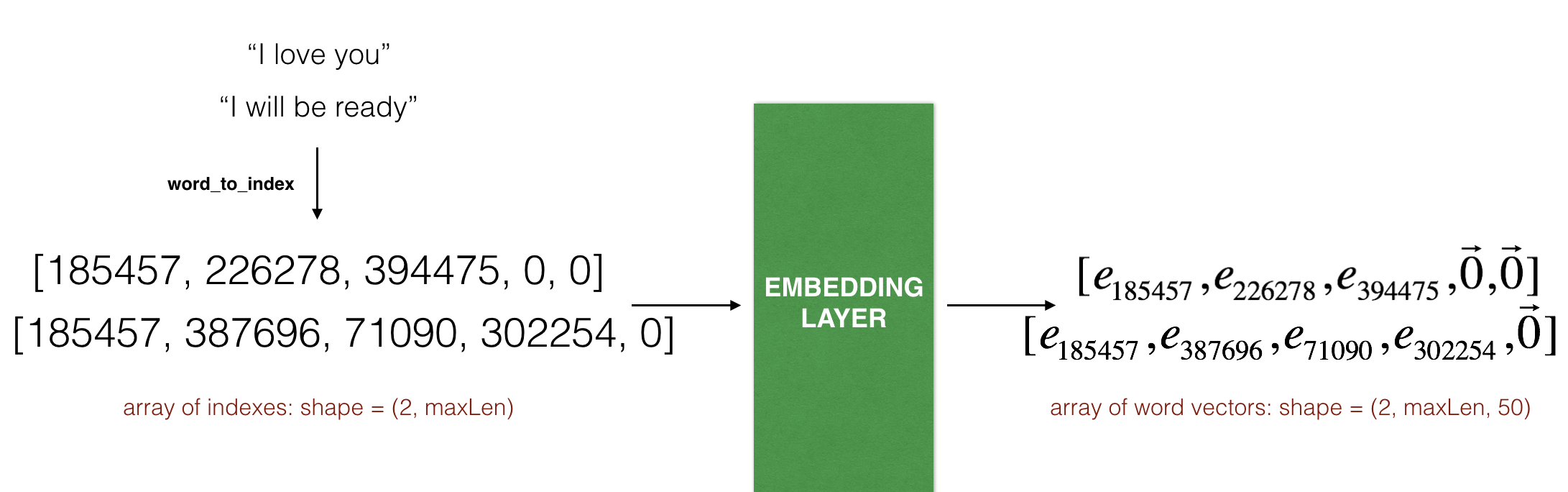
So, the first step we want to do is to convert all our training sentences into lists of indices, and then zero-pad all these lists so that their length is the length of the longest sentence.
Also, we know that the largest integer (i.e. word index) in the input should be no larger than the vocabulary size.
The layer outputs an array of shape (batch size, max input length, dimension of word vectors).

Let's make a function to convert our sentence array into indices array, so that it can be fed into the Embedding layer.

def sentences_to_indices(X, word_to_index, max_len):
    """
    Converts an array of sentences (strings) into an array of indices corresponding to words in the sentences.
    The output shape should be such that it can be given to `Embedding()` (described in Figure 4). 
    
    Arguments:
    X -- array of sentences (strings), of shape (m, 1)
    word_to_index -- a dictionary containing the each word mapped to its index
    max_len -- maximum number of words in a sentence. You can assume every sentence in X is no longer than this. 
    
    Returns:
    X_indices -- array of indices corresponding to words in the sentences from X, of shape (m, max_len)
    """
    
    m = X.shape[0]                                   # number of training examples
    
    ### START CODE HERE ###
    # Initialize X_indices as a numpy matrix of zeros and the correct shape (≈ 1 line)
    X_indices = np.zeros((m,max_len))
    
    for i in range(m):                               # loop over training examples
        
        # Convert the ith training sentence in lower case and split is into words. You should get a list of words.
        sentence_words = [w.lower() for w in X[i].split()]
        
        # Initialize j to 0
        j = 0
        
        # Loop over the words of sentence_words
        for w in sentence_words:
            # Set the (i,j)th entry of X_indices to the index of the correct word.
            X_indices[i, j] = word_to_index[w]
            # Increment j to j + 1
            j = j+1
            
    ### END CODE HERE ###
    
    return X_indices

Let's build the Embedding() layer in Keras, using pre-trained word vectors. After this layer is built, we will pass the output of sentences_to_indices() to it as an input, and the Embedding() layer will return the word embeddings for a sentence.

What we will do is:

• We will initialize the embedding matrix as a numpy array of zeros with the correct shape.
• Then, fill in the embedding matrix with all the word embeddings extracted from word_to_vec_map.
• Define the Keras embedding layer. We will make this layer non-trainable, by setting trainable = False when calling Embedding(). If we were to set trainable = True, then it will allow the optimization algorithm to modify the values of the word embeddings.
• Set the embedding weights to be equal to the embedding matrix.

So our function takes in the pre-trained Glove 50 dimensional vectors and creates an Embedding() layer.

def pretrained_embedding_layer(word_to_vec_map, word_to_index):
    """
    Creates a Keras Embedding() layer and loads in pre-trained GloVe 50-dimensional vectors.
    
    Arguments:
    word_to_vec_map -- dictionary mapping words to their GloVe vector representation.
    word_to_index -- dictionary mapping from words to their indices in the vocabulary (400,001 words)

    Returns:
    embedding_layer -- pretrained layer Keras instance
    """
    
    vocab_len = len(word_to_index) + 1                  # adding 1 to fit Keras embedding (requirement)
    emb_dim = word_to_vec_map["cucumber"].shape[0]      # define dimensionality of your GloVe word vectors (= 50)
    
    ### START CODE HERE ###
    # Initialize the embedding matrix as a numpy array of zeros of shape (vocab_len, dimensions of word vectors = emb_dim)
    emb_matrix = np.zeros((vocab_len,emb_dim))
    
    # Set each row "index" of the embedding matrix to be the word vector representation of the "index"th word of the vocabulary
    for word, index in word_to_index.items():
        emb_matrix[index, :] = word_to_vec_map[word]

    # Define Keras embedding layer with the correct output/input sizes, make it trainable. Use Embedding(...). Make sure to set trainable=False. 
    embedding_layer = Embedding(input_dim = vocab_len, output_dim = emb_dim, trainable = False)
    ### END CODE HERE ###

    # Build the embedding layer, it is required before setting the weights of the embedding layer. Do not modify the "None".
    embedding_layer.build((None,))
    
    # Set the weights of the embedding layer to the embedding matrix. Your layer is now pretrained.
    embedding_layer.set_weights([emb_matrix])
    
    return embedding_layer

4. Model
   Our model takes as input an array of sentences of shape (m, max_len, ) defined by input_shape and it should output a softmax probability vector of shape (m, C = 5).

def Emojify(input_shape, word_to_vec_map, word_to_index):
    """
    Function creating the Emojify-v2 model's graph.
    
    Arguments:
    input_shape -- shape of the input, usually (max_len,)
    word_to_vec_map -- dictionary mapping every word in a vocabulary into its 50-dimensional vector representation
    word_to_index -- dictionary mapping from words to their indices in the vocabulary (400,001 words)

    Returns:
    model -- a model instance in Keras
    """
    
    ### START CODE HERE ###
    # Define sentence_indices as the input of the graph, it should be of shape input_shape and dtype 'int32' (as it contains indices).
    sentence_indices = Input(input_shape,dtype = 'int32')
    
    # Create the embedding layer pretrained with GloVe Vectors (≈1 line)
    embedding_layer = pretrained_embedding_layer(word_to_vec_map, word_to_index)
    
    # Propagate sentence_indices through your embedding layer, you get back the embeddings
    embeddings = embedding_layer(sentence_indices) 
    
    # Propagate the embeddings through an LSTM layer with 128-dimensional hidden state
    # Be careful, the returned output should be a batch of sequences.
    X = LSTM(128,return_sequences = True)(embeddings)
    # Add dropout with a probability of 0.5
    X = Dropout(0.5)(X)
    # Propagate X trough another LSTM layer with 128-dimensional hidden state
    # Be careful, the returned output should be a single hidden state, not a batch of sequences.
    X = LSTM(128,return_sequences = False)(X)
    # Add dropout with a probability of 0.5
    X = Dropout(0.5)(X)
    # Propagate X through a Dense layer with softmax activation to get back a batch of 5-dimensional vectors.
    X = Dense(5)(X)
    # Add a softmax activation
    X = Activation('softmax')(X)
    
    # Create Model instance which converts sentence_indices into X.
    model = Model(inputs = sentence_indices,outputs=X)
    
    ### END CODE HERE ###
    
    return model

5. Let's create our model and compile it

model = Emojify((maxLen,), word_to_vec_map, word_to_index)
model.compile(loss='categorical_crossentropy', optimizer='adam', metrics=['accuracy'])

6. Training of Model
   It's time to train our model. Our Emojifier model takes as input an array of shape (m, max_len) and outputs probability vectors of shape (m, number of classes). We thus have to convert X_train (array of sentences as strings) to X_train_indices (array of sentences as list of word indices), and Y_train (labels as indices) to Y_train_oh (labels as one-hot vectors).

X_train_indices = sentences_to_indices(X_train, word_to_index, maxLen)
Y_train_oh = convert_to_one_hot(Y_train, C = 5)

Now, we will start training our model.

model.fit(X_train_indices, Y_train_oh, epochs = 50, batch_size = 32, shuffle=True)

7. Model evaluation

X_test_indices = sentences_to_indices(X_test, word_to_index, max_len = maxLen)
Y_test_oh = convert_to_one_hot(Y_test, C = 5)
loss, acc = model.evaluate(X_test_indices, Y_test_oh)
print()
print("Test accuracy = ", acc)

Output:
Test accuracy = 0.82 (approx)

To appreciate the performance of our LSTM model, let's look at an interesting example, that actually sets LSTM apart from statistical word embedding models or even simple RNN models.
Input: "Not feeling happy"
Output:

Had we used simpler models, the output would have been a happy face!

Final thoughts

• RNN’s are good for processing sequence data for predictions but suffers from short-term memory.
• RNN’s have the benefit of training faster and uses less computational resources.That’s because there are fewer tensor operations to compute.
• LSTM cells are variants of RNN capable of handling long term dependencies.

Keep learning and keep sharing!