
Open-Source Internship opportunity by OpenGenus for programmers. Apply now.
To solve Jigsaw Puzzles using Machine Learning, we have explored the paper "Unsupervised Learning of Visual Representations by Solving Jigsaw Puzzles". The paper describes a convolutional neural network (CNN) that aims to solve a pretext task, solving Jigsaw puzzles without manual labelling, and then to solve object classification and detection tasks.
The research in the paper has been done by Mehdi Noroozi and Paolo Favaro from University of Bern, Switzerland.
This paper introduces a new self-supervised task, the Jigsaw reassembly problem, which performs well when transferred to detection and classification tasks. The goal of training a computer to solve Jigsaw puzzles is to teach it that an object is composed of several parts and for the computer to identify what these parts are. The benefits of this method are the short amount of taken (2.5 days compared to 4 weeks in the task proposed by Doersch et al.). Chromatic aberration does not have to be handled and there is no need to build robustness to pixelation. The features are highly transferable and is currently the top performer for an unsupervised method.
This work is classified as representation/feature learning, an unsupervised learning problem that tries to build intermediate representations of data so as to solve machine learning tasks. It is also an example of transfer learning, as the skills learned by the system in solving the Jigsaw puzzle can be applied to object classification and detection.
This model includes pre-training and fine-tuning. The feature learning obtained with the Jigsaw puzzle solver is the pre-training and fine-tuning involves updating weights obtained during pre-training to solve other tasks.
Unsupervised Learning Method
This model highlights the use of a self-supervised training model as an improvement on a typical unsupervised learning method. While historically, labelled data have been used to train a parametric model, unsupervised learning methods are now gaining momentum as they do not require manually labelled data and are hence less costly. Instead, self-supervised learning exploits different labels that are freely available alongside visual data and they are used as intrinsic reward signals for learning general-purpose features.
This led to three different methods of unsupervised learning. Two of them exploit multiple images with a temporal or viewpoint transformation by using object correspondence obtained through tracking in videos (Wang and Gupta), and ego-motion information obtained by a mobile agent such as the Google car (Agrawal et al.) respectively. While biological agents may employ these methods and integrate further additional sensory motion, single snapshots can carry more information. The third uses the relative spatial co-location of patches in images as a label and only uses single images as the training set (Doersch et al.).
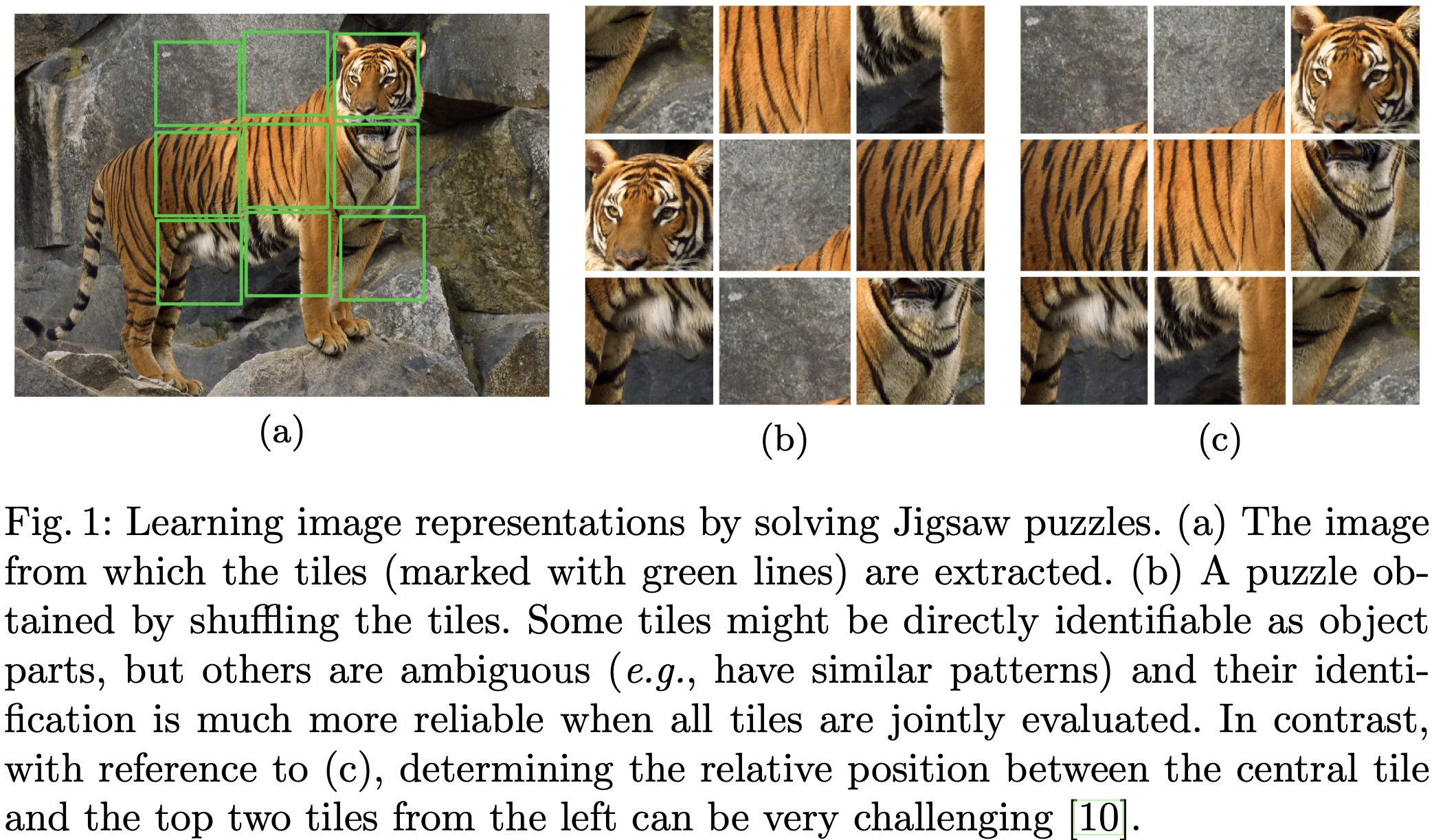
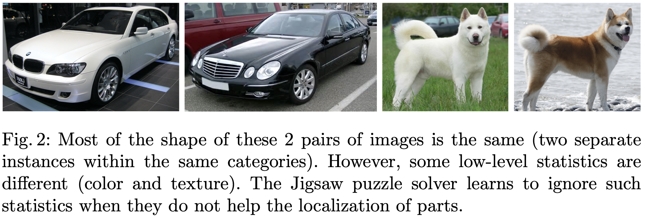
The Jigsaw puzzle method observes all the tiles simultaneously, allowing the trained network to insect all ambiguity sets and hopefully reduce it to a singleton. It ignores low-level similarities between tiles such as colour or texture when they do not help localise parts, but focuses on their differences instead.
This CFN shows that it is possible for self-supervising learning to match the performance of supervised learning, which can cut costs by abolishing the need for costly human annotation.
Solving the Jigsaw Puzzle
The model uses a context-free network, where data flow of each patch is explicitly separated until the fully connected layer, which is the only layer where context is handled. Compared to AlexNet, the CFN is used despite having a 0.3% olower accuracy (The CFN yields 57.1% top-1 accuracy compared with 57.4% for AlexNet), because it is significantly more compact, using 27.5M parameters compared to AlexNet's 61M.
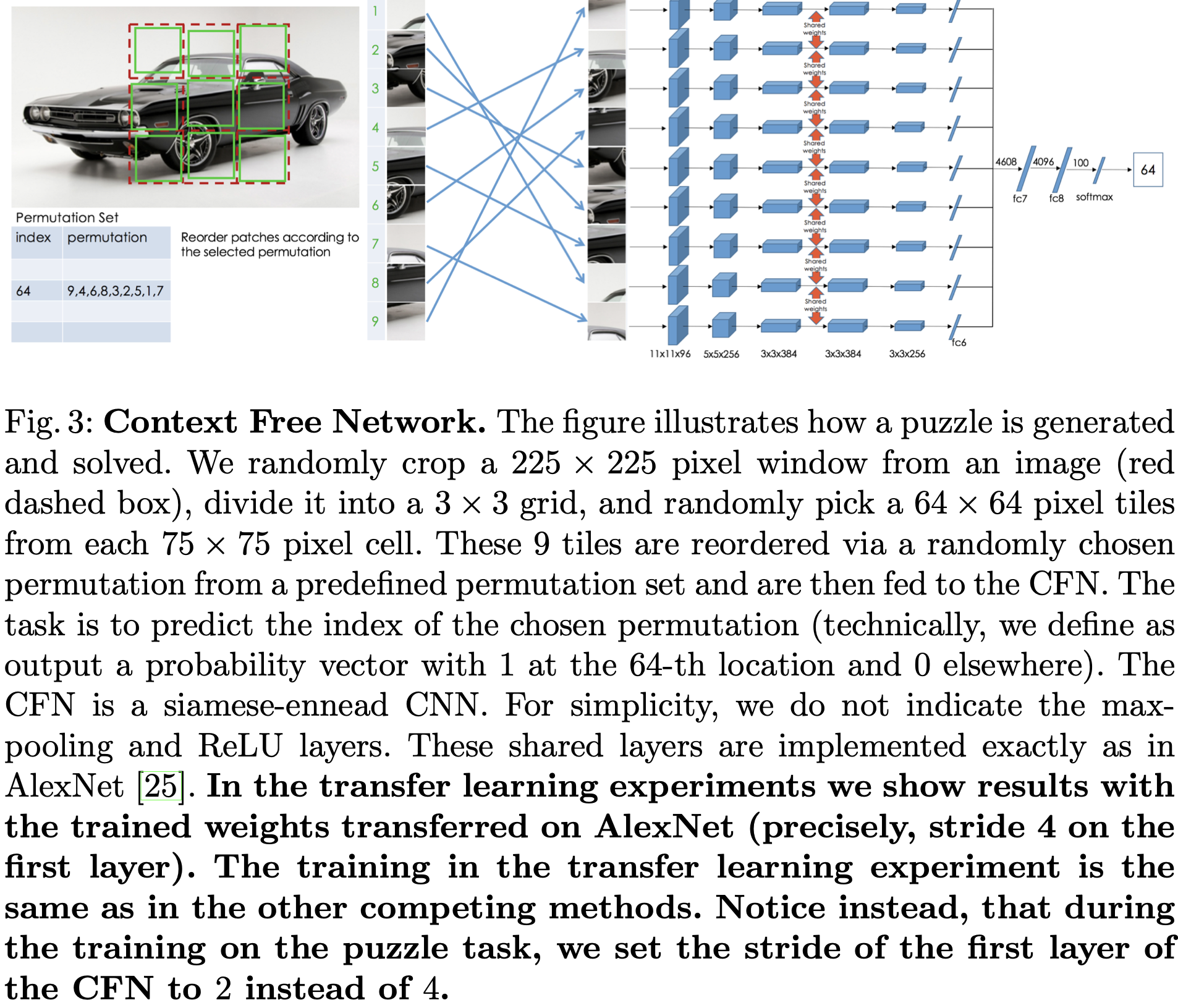
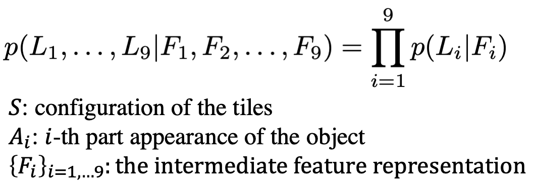
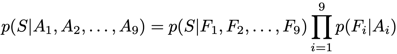
To solve the task, a set of Jigsaw puzzle permutations are defined and each entry is assigned an index. One permutation is randomly picked, 9 input patches are rearranged according to that permutation, and the CFN aims to return a vector with the probability value for each index. This output can be considered as the conditional probability density function of the spatial arrangement of object parts, which can be represented as follows.
The CFN was implemented by using stochastic gradient descent without batch normalisation on one Titan X GPU. For transfer learning, learned features were used as pre-trained weights for classification, detection and semantic segmentation tasks. A new benchmark was also developed to evaluate the method for machine learning.
Avoiding shortcuts
General shortcut issues refer to the development of the learning system to solve the pre-text task, being the Jigsaw puzzle, instead of the target tasks of object classification, detection and segmentation.
Feature association with positions
For one, the CFN may accidentally learn to associate features with absolute positions if only 1 Jigsaw puzzle is generated per image. The following equation illustrates how the conditional pdf can be factorised into independent terms by writing the configuration S as a list of tile positions.
This shortcut can be avoided by feeding the CFN multiple Jigsaw puzzles of the same image, making sure that tiles are shuffled as much as possible and have adequately large average Hamming distance, ensuring that the same tile can be assigned to multiple positions within the grid and avoiding the correlation of an absolute position.
Low level statistics
These can include the mean and start deviation of the pixel intensities, allowing the model to find the arrangement of the patches. Hence the mean and standard deviation is normalised for every patch.
Edge continuity
Another shortcut can be the CFN learns to notice edge continuity and pixel intensity distribution. The CFN does not learn low-level statistics by mitigating this issue. This includes leaving random gaps between tiles between the size of 0 to 22 pixels by resizing input images and cropping a random region. Selecting 64x64 pixel tiles randomly from the 85x85 pixel cells allows for a 21 pixel gap between tiles.
Chromatic aberration
A third shortcut can be due to chromatic aberration, which is a relative spacial shift between colour channels that increases from the center images to the borders, which helps the network estimate the tiles. This is resolved by cropping the central squre of the original image and resizing it, training with both colour and grayscale and jittering colour channels and using greyscale images.
The dataset was kept small by using Caffe (see reference 3 for details) to choose random image patches and permutations, allowing for efficient training. In more tangible figures, each image could generate 69 different puzzles on average.
Ablation studies
Ablation studies were performed to examine the impact of each component training under different scenarios.
The permutation set had a signification impact on the ambiguity of the tasks, as closer permutations made the puzzle task more challenging and ambiguous. One criteria is cardinality, where a larger number of permutations causes the training on the Jigsaw task to become increasingly difficult, but leads to an improvement in the performance of the detection task.
The average Hamming distance between permutations positively correlates with the difficulty of the Jigsaw puzzle reassembly task. A higher average Hamming distance leads to less Jigsaw puzzle solving error and lower object detection errors when fine tuning is used for transfer learning. The permutation set is generated iteratively with a greedy algorithm.
The minimum Hamming distance is increased by removing similar permutations in a maximal set with 100 initial entries, as the minimum distance makes the task less ambiguous.
Overall, the best performing permutation set is a trade off between the number of permutations and their dissimilarity from each other, which leads to the conclusion that a good self-supervised task is neither simple nor ambiguous.
CFN filter activations and image retrieval
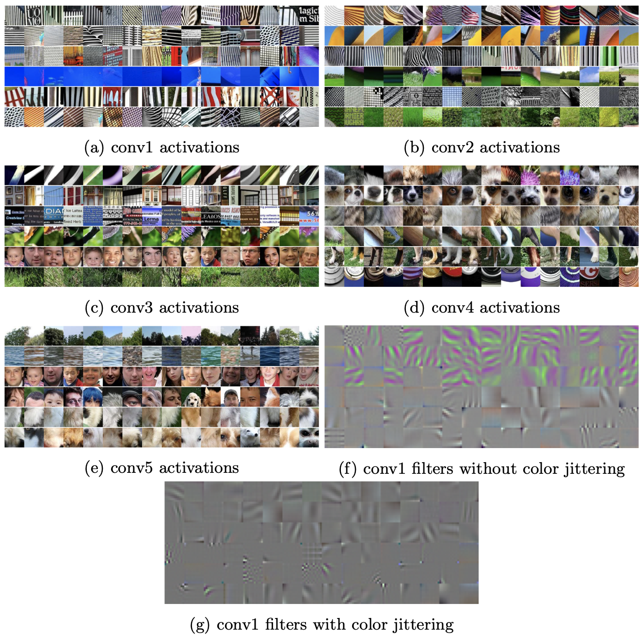
The units at each layer of this CFN can be considered object part detectors. By dissecting the CFN into its layers and by evaluating the features qualitatively with a simple image ranking, the top activations of the layers trained in the CFN can be visualised.
The below figure shows how the conv1 and conv2 layers specialise in texture, the conv3 specialises in face and part detectors, conv4 includes a larger number of part detectors and the fifth layer can detect parts and scenes.
References
- Agrawal, P., Carreira, J., Malik, J.: Learning to see by moving. ICCV (2015)
- Doersch, C., Gupta, A., Efros, A.A.: Unsupervised visual representation learning by context prediction. ICCV (2015)
- Jia, Y., Shelhamer, E., Donahue, J., Karayev, S., Long, J., Girshick, R., Guadar- rama, S., Darrell, T.: Caffe: Convolutional architecture for fast feature embedding. ACM-MM (2014)
- Wang, X., Gupta, A.: Unsupervised learning of visual representations using videos. ICCV (2015)
With this article at OpenGenus, you must have the complete idea of solving jigsaw puzzles using a Machine Learning approach. Enjoy.