
Open-Source Internship opportunity by OpenGenus for programmers. Apply now.
Reading time: 35 minutes | Coding time: 10 minutes
In this article, we will demonstrate how we can use K-Nearest Neighbors algorithm for classifying input text into a category of 20 news groups. We will go through these sub-topics:
- Basic overview of K Nearest Neighbors (KNN) as a classifier
- How KNN works in text?
- Code demonstration of Text classification using KNN
K-Nearest Neighbors
- Let's first understand the term neighbors here. The closeness/ proximity amongst samples of data determines their neighborhood. There are several ways to calculate the proximity/distance between data points depending on the problem to solved. Most familiar and popular is straight-line distance (Euclidean Distance).
- Generally, neighbors share similar characteristics and behavior that's why they can be treated as they belong to the same group.
- This is the main idea of this simple supervised learning classification algorithm.
- Now, for the K in KNN algorithm that is we consider the K-Nearest Neighbors of the unknown data we want to classify and assign it the group appearing majorly in those K neighbors. For K=1, the unknown/unlabeled data will be assigned the class of its closest neighbor.
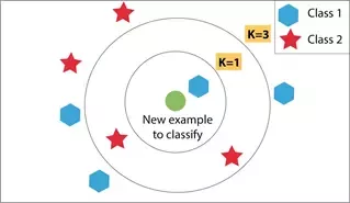
- We want to select a value of K that is reasonable and not something too big (it will predict the class having majority among all data samples) or something too small.
Let's see how this works on this example dataset of music fans,
| Name | Age | Gender | Music Band |
|---|---|---|---|
| Amantha | 19 | F | Coldplay |
| Brendon | 23 | M | Coldplay |
| Nate | 24 | M | LinkinPark |
| Sam | 30 | M | LininPark |
| Betty | 16 | F | Coldplay |
| Christine | 18 | F | LinkinPark |
| Gin | 22 | F | LinkinPark |
| Ken | 18 | M | Coldplay |
| Susy | 15 | F | Coldplay |
Now, we have a person named Gary who is a 23 year male and we want to predict which band will he like more. Here's how we can use the KNN algorithm,
Firstly we'll have to translate gender to some numbers for the distance/ proximity relation needed for finding neighbors.
We do this by translating male->0 and female->1.
For each data entry distance is calculated from Gary and distance for ith data is given as,
| Name | Age | Gender | Music Band | Distance^2 |
|---|---|---|---|---|
| Amantha | 19 | 1 | Coldplay | 17 |
| Brendon | 23 | 0 | Coldplay | 0 |
| Nate | 24 | 0 | LinkinPark | 1 |
| Sam | 30 | 0 | LininPark | 49 |
| Betty | 16 | 1 | Coldplay | 50 |
| Christine | 18 | 1 | LinkinPark | 26 |
| Gin | 22 | 1 | LinkinPark | 2 |
| Ken | 18 | 0 | Coldplay | 25 |
| Susy | 15 | 1 | Coldplay | 65 |
Let's say, K=3 then the K-Nearest Neighbors are
| Name | Age | Gender | Music Band | Distance^2 |
|---|---|---|---|---|
| Brendon | 23 | 0 | Coldplay | 0 |
| Nate | 24 | 0 | LinkinPark | 1 |
| Gin | 22 | 1 | LinkinPark | 2 |
LinkinPark is followed more by Gary's Neighbors so we predict that Gary will also like LinkinPark more than Coldplay.
How K-NN works in text?
The major problem in classifying texts is that they are mixture of characters and words. We need numerical representation of those words to feed them into our K-NN algorithm to compute distances and make predictions.
One way of doing that numerical representation is bag of words with tf-idf(Term Frequency - Inverse document frequency). If you have no idea about these terms, you should check out our previous guide about them before moving ahead.
Let's say we have our text data represented in feature vectors as,
| ID | Class | Word1 | Word2 | Word3 |
|---|---|---|---|---|
| 1 | 0 | 2 | 0 | 3 |
| 2 | 1 | 3 | 1 | 1 |
| 3 | 1 | 0 | 3 | 2 |
| 4 | 0 | 1 | 2 | 1 |
We will have a feature vector of unlabeled text data and it's distance will be calculated from all these feature vectors of our data-set. Out of them, K-Nearest vectors will be selected and the class having maximum frequency will be labeled to the unlabeled data.
Making it Work
Setup
For this task, we'll need:
- Python: To run our script
- Pip: Necessary to install Python packages
Now we can install some packages using pip, open your terminal and type these out.
pip install numpy
pip install sklearn
Numpy: Useful mathematical functions
Sklearn: Machine learning tools for python
Code
Let's import the libraries for the task,
import numpy as np
from sklearn.datasets import fetch_20newsgroups
from sklearn.feature_extraction.text import CountVectorizer
from sklearn.feature_extraction.text import TfidfTransformer
from sklearn.neighbors import KNeighborsClassifier
from sklearn.pipeline import Pipeline
Now, we'll get the dataset ready,
from sklearn.datasets import fetch_20newsgroups
Now, we define the categories we want to classify our text into and define the training data set using sklearn.
# We defined the categories which we want to classify
categories = ['rec.motorcycles', 'sci.electronics',
              'comp.graphics', 'sci.med']

# sklearn provides us with subset data for training and testing
train_data = fetch_20newsgroups(subset='train',
                                categories=categories, shuffle=True, random_state=42)

print(train_data.target_names)

print("\n".join(train_data.data[0].split("\n")[:3]))
print(train_data.target_names[train_data.target[0]])

# Let's look at categories of our first ten training data
for t in train_data.target[:10]:
    print(train_data.target_names[t])
['comp.graphics', 'rec.motorcycles', 'sci.electronics', 'sci.med']
From: kreyling@lds.loral.com (Ed Kreyling 6966)
Subject: Sun-os and 8bit ASCII graphics
Organization: Loral Data Systems
comp.graphics
comp.graphics
comp.graphics
rec.motorcycles
comp.graphics
sci.med
sci.electronics
sci.electronics
comp.graphics
rec.motorcycles
sci.electronics
Here we are pre-processing on text and generating feature vectors of token counts and then transform into tf-idf representation.
Consider a document containing 100 words wherein the word ‘car’ appears 7 times.
The term frequency (tf) for phone is then (7 / 100) = 0.07. Now, assume we have 1 million documents and the word car appears in one thousand of these. Then, the inverse document frequency (i.e., IDF) is calculated as log(10,00,000 / 100) = 4. Thus, the Tf-IDF weight is the product of these quantities: 0.07 * 4 = 0.28.
i.e. Apply Vectorizer=> Transformer.
# Builds a dictionary of features and transforms documents to feature vectors and convert our text documents to a
# matrix of token counts (CountVectorizer)
count_vect = CountVectorizer()
X_train_counts = count_vect.fit_transform(train_data.data)

# transform a count matrix to a normalized tf-idf representation (tf-idf transformer)
tfidf_transformer = TfidfTransformer()
X_train_tfidf = tfidf_transformer.fit_transform(X_train_counts)
We fit our Multinomial Naive Bayes classifier on train data to train it.
knn = KNeighborsClassifier(n_neighbors=7)

# training our classifier ; train_data.target will be having numbers assigned for each category in train data
clf = knn.fit(X_train_tfidf, train_data.target)

# Input Data to predict their classes of the given categories
docs_new = ['I have a Harley Davidson and Yamaha.', 'I have a GTX 1050 GPU']
# building up feature vector of our input
X_new_counts = count_vect.transform(docs_new)
# We call transform instead of fit_transform because it's already been fit
X_new_tfidf = tfidf_transformer.transform(X_new_counts)
Predict the output of our input text by using the classifier we just trained.
# predicting the category of our input text: Will give out number for category
predicted = clf.predict(X_new_tfidf)

for doc, category in zip(docs_new, predicted):
    print('%r => %s' % (doc, train_data.target_names[category]))
'I have a Harley Davidson and Yamaha.' => rec.motorcycles
'I have a GTX 1050 GPU' => sci.med
We now finally evaluate our model by predicting the test data. Also, you'll see how to do all of the tasks of vectorizing, transforming and classifier into a single compund classifier using Pipeline.
# We can use Pipeline to add vectorizer -> transformer -> classifier all in a one compound classifier
text_clf = Pipeline([
    ('vect', CountVectorizer()),
    ('tfidf', TfidfTransformer()),
    ('clf', knn),
])
# Fitting our train data to the pipeline
text_clf.fit(train_data.data, train_data.target)

# Test data
test_data = fetch_20newsgroups(subset='test',
                               categories=categories, shuffle=True, random_state=42)
docs_test = test_data.data
# Predicting our test data
predicted = text_clf.predict(docs_test)
print('We got an accuracy of',np.mean(predicted == test_data.target)*100, '% over the test data.')
We got an accuracy of 82.36040609137056 % over the test data.
Useful Insights
In K-NN, we need to tune in the K parameter based on validation set. The value of K will smooth out the boundaries between classes. Generally, the value of K is taken to be as $\sqrt{n}$, where n = number of data samples.
The overhead of calculating distances for every data whenever we want to predict is really costly. So, K-NN is not useful in real-time prediction.
In Naive Bayes, conditional independence is assumed in real data and it attempts to approximate the optimal soltuion. Naive Bayes is a quick classifier.
K-NN should be preferred when the data-set is relatively small. Also, you must scale all the features to normalized measure because we don't want the units of one feature influence significantly over the units of other feature.