Reading time: 40 minutes | Coding time: 15 minutes

Topic Modeling is a mathematical process of obtaining abstract topics for a corpus based on the words present in each of the document. It is a kind of unsupervised machine learning model trying to find the text correlation between the documents. There are various models available to perform topic modeling like Latent Dirichlet Allocation, Latent Semantic Analysis etc In this article, we will be looking at the functioning and working of Latent Semantic Analysis. We will also be looking at the mathematics behind the method.

Latent Semantic Analysis

Latent Semantic Model is a statistical model for determining the relationship between a collection of documents and the terms present n those documents by obtaining the semantic relationship between those words. Here we form a document-term matrix from the corpus of text. Each row in the column represent unique words in the document and each column represent a single document. The process is achieved by Singular Value Decomposition.

Before diving into the mathematics behind the model, let us first look at some key definitions that would let us have clear understanding of the concepts behind LSA.

Term document matrix is the frequency of occurance of words in a collection of documents. Here, the rows represent the documents in the corpus and the columns represent the unique words in the corpus.

A Singular matrix is a matrix where its determinant does not exist or it is not invertible.

Eigen vector represents the direction in which the matrix or vector is aligned due to the operations performed on it. Eigen values represnts the scale by which the vector is streched in that direction.

Orthonomal matrix is a matrix where each colun vectoe has unit length and is orthogonal to all other columns ( i.e.)their dot product is zero.

Math behind the Model

Latent Semantic Analysis works on the basis of Singular Value Decomposition. It is a method of factorizing a matrix into three matrices. Let us consider a matrix A which is to be factorized. It is then factorized into three unique matrices U, L and V where U and V are orthonormal matrices and L is a singular matrix.

For example, look at the below matrices.

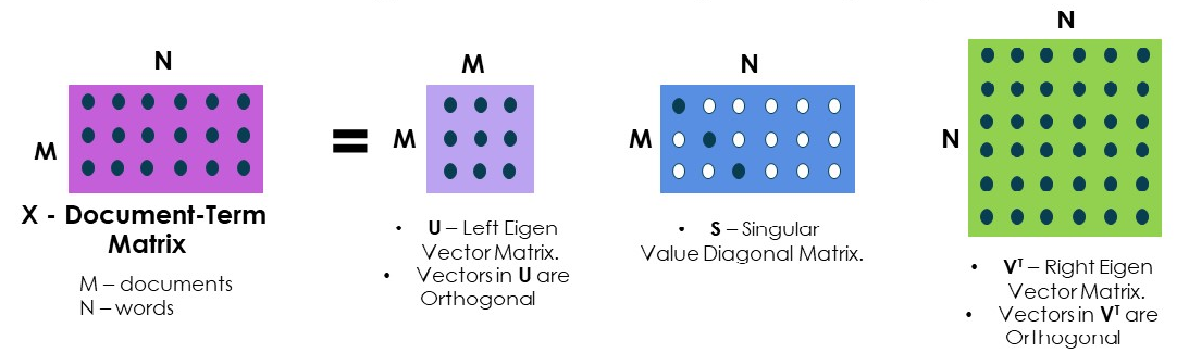
X is the term-document matrix which consists of all the words present in each of the documents. U and V Transpose Matrices are orthonormal matrices where each row is a orthogonal vectors.

S is a singular value diagonal matrix with its eigen values present along the diagonal.

Each row of the matrix V Transpose represents the topics and the values for a particular topic in each columns represents the importance and relationship of that word in the corresponding document [Note: Each column represents a unique document].

Hence, V is the matrix that is central of topic modeling and can be used for assigning topics to a document and other applications.

Implementation

Python implementation of Singular Value Decomposition is given below. We will use the scipy package of SVD to perform the operation.

First let us import the required packages and define our A matrix.

import numpy as np
from scipy.linalg import svd

A = np.array([[1, 2], [3, 4], [5, 6]])
print(A)

Now, let us perform Singular Value Decomposition to obtain our required resultant matrices by factorization.

U, S, VT = svd(A)
print(U)
print(S)
print(VT)

Text Analysis

Now let us have a clear understanding of what this method is by having a real-time project go-through. Here, we will perform Latent Semantic Analysis to identify the cluster of topics for a given corpus.

First of all, let us import all the required packages to perform the project.

import re
import numpy as np
import pandas as pd
from scipy import linalg, spatial
from sklearn.cluster import KMeans
from sklearn.decomposition import PCA, SparsePCA, TruncatedSVD
from sklearn.feature_extraction.text import (CountVectorizer, TfidfTransformer, TfidfVectorizer)
from sklearn.cluster import KMeans

from sklearn.utils.extmath import randomized_svd

from nltk.tokenize import word_tokenize
from nltk.corpus import stopwords

Now, we will import the text we are going to analyze. The text is an extract about Robert Downey Jr. from wikipedia. Only a small extract of the text is used to clearly understand the working process. This process can be scaled to large texts using request and BeautifulSoup packages.

corpus = [

          "With all of the critical success Downey had experienced throughout his career, he had not appeared in a blockbuster film. That changed in 2008 when Downey starred in two critically and commercially successful films, Iron Man and Tropic Thunder. In the article Ben Stiller wrote for Downey's entry in the 2008 edition of The Time 100, he offered an observation on Downey's commercially successful summer at the box office.",
          "On June 14, 2010, Downey and his wife Susan opened their own production company called Team Downey. Their first project was The Judge.",
          "Robert John Downey Jr. is an American actor, producer, and singer. His career has been characterized by critical and popular success in his youth, followed by a period of substance abuse and legal troubles, before a resurgence of commercial success in middle age.",
          "In 2008, Downey was named by Time magazine among the 100 most influential people in the world, and from 2013 to 2015, he was listed by Forbes as Hollywood's highest-paid actor. His films have grossed over $14.4 billion worldwide, making him the second highest-grossing box-office star of all time."
          
          ]

stop_words = set(stopwords.words('english'))

We have four documents in this corpus. We have also removed the stopwords which includes some of the most common repeating words which does not contribute to the meaning of the sentences.

Now, we will split the whole document into individual words using the tokenizer. The individual tokens are then complied into a python dictionary filtered_text.

filtered_document= []
filtered_text = []

for document in corpus:
    
    clean_document = " ".join(re.sub(r"[^A-Za-z \—]+", " ", document).split())
    
    document_tokens = word_tokenize(clean_document)

    for word in document_tokens:
        if word not in stop_words:
            filtered_document.append(word)

    filtered_text.append(' '.join(filtered_document))

Now, we will form a word frequency matrix to count the usage of different words in different documents in the corpus.

vectorizer = CountVectorizer()

counts_matrix = vectorizer.fit_transform(filtered_text)

feature_names = vectorizer.get_feature_names()

count_matrix_df = pd.DataFrame(counts_matrix.toarray(), columns=feature_names)
count_matrix_df.index = ['Document 1','Document 2','Document 3','Document 4']

print("Word frequency matrix: \n", count_matrix_df)

The output of this code prints a matrix which shows the frequency of occurance of every word in each document.

We will view the featured names obtained and we use Kmeans algorithm to identify the closely related words by unsupervised machine learning algorithm.

vectorizer = TfidfVectorizer(stop_words=stop_words,max_features=10000, max_df = 0.5,
                                    use_idf = True,
                                    ngram_range=(1,3))

X = vectorizer.fit_transform(filtered_text)
print(X.shape)
print(feature_names)

num_clusters = 4

km = KMeans(n_clusters=num_clusters)
km.fit(X)
    
clusters = km.labels_.tolist()
print(clusters)

Now let us generate the topics for the corpus using SVD.

U, Sigma, VT = randomized_svd(X, n_components=10, n_iter=100, random_state=122)

svd_model = TruncatedSVD(n_components=2, algorithm='randomized', n_iter=100, random_state=122)

svd_model.fit(X)
    
print(U.shape)

for i, comp in enumerate(VT):
    terms_comp = zip(feature_names, comp)
    sorted_terms = sorted(terms_comp, key= lambda x:x[1], reverse=True)[:7]
    print("Cluster "+str(i)+": ")
    for t in sorted_terms:
        print(t[0])
    print(" ")

The result obtained from the program is attached below. This shows how the topics are obtained based on the semantic relationship between words.

Cluster 0: 
american
age
actor
article
ben
billion
called

Cluster 1: 
actor
article
ben
billion
called
career
changed

Cluster 2: 
american
age
actor
among
appeared
blockbuster
box

Cluster 3: 
american
actor
abuse
article
ben
billion
called

In order to get a clear picture of what is happening, let us look at the structure of the matrices generated.

The orthonormal matrix VT obtained is given below:

[[ 0.10691121  0.10691121  0.10691121  0.14737057  0.05131756  0.05131756
   0.10691121  0.10691121  0.10691121  0.05131756  0.05131756  0.10691121
   0.10691121  0.10691121  0.05131756  0.05131756  0.05131756  0.05131756
   0.05131756  0.05131756  0.05131756  0.10691121  0.10691121  0.10691121
   0.10691121  0.10691121  0.10691121  0.10691121  0.10691121  0.10691121
   0.10691121  0.10691121  0.10691121  0.05131756  0.05131756  0.05131756
   0.05131756  0.10691121  0.10691121  0.10691121  0.05131756  0.05131756
   0.05131756  0.05131756  0.05131756  0.05131756  0.05131756  0.05131756
   0.05131756  0.10263512  0.05131756  0.05131756  0.05131756  0.05131756
   0.05131756  0.05131756  0.05131756  0.05131756  0.05131756  0.05131756
   0.10691121  0.10691121  0.10691121  0.10691121  0.10691121  0.10691121
   0.10691121  0.10691121  0.10691121  0.10691121  0.10691121  0.05131756
   0.05131756  0.05131756  0.05131756  0.05131756  0.05131756  0.05131756
   0.05131756  0.05131756  0.10691121  0.10691121  0.05131756  0.05131756
   0.05131756  0.05131756  0.05131756  0.05131756  0.05131756  0.05131756
   0.05131756  0.05131756  0.05131756  0.05131756  0.10691121  0.10691121
   0.10691121  0.10691121  0.10691121  0.10691121  0.10691121  0.10691121
   0.10691121  0.10691121  0.10691121  0.10691121  0.10691121  0.10691121
   0.10691121  0.10691121  0.05131756  0.05131756  0.05131756  0.10691121
   0.10691121  0.10691121  0.05131756  0.05131756  0.10691121  0.10691121
   0.10691121  0.10691121  0.10691121  0.10691121  0.10691121  0.05131756
   0.05131756  0.10691121  0.10691121  0.10691121  0.05131756  0.05131756
   0.05131756  0.05131756  0.05131756  0.05131756  0.10691121  0.10691121
   0.10691121]
    ... 3 more such rows
]

The orthonormal matrix U is given below.

[[ 0.00000000e+00  0.00000000e+00  0.00000000e+00  1.00000000e+00]
 [ 0.00000000e+00  2.91421830e-17  1.00000000e+00  0.00000000e+00]
 [ 7.07106781e-01  7.07106781e-01  1.11022302e-16  0.00000000e+00]
 [ 7.07106781e-01 -7.07106781e-01  0.00000000e+00  0.00000000e+00]]

Finally the singualar value matrix Sigma thus obtained is given below.

[ 1.27182939e+00  6.18425417e-01  1.38136902e-17 -0.00000000e+00]

Conclusion

In this article, we have walked through Latent Semantic Analysis and its python implementation. we have also looked at the Singular Value Decomposition mathematical model.