Reading time: 40 minutes | Coding time: 20 minutes

Support vector machines (SVMs) are a particularly powerful and flexible class of supervised algorithms for both classification and regression.

After reading this article you will get familiar with the following terms in detail about SVM:-

1. Introduction
2. Intuition behind SVMs
3. Mathematical explanation
   • Kernel trick
   • Constrained optimization
4. Implementation with python
5. Applications of SVM in the real world

1. Introduction:-

Support Vector Machines (SVMs) are regarding a novel way of estimating a non-linear function by using a limited number of training examples.

• Getting stuck in local minima is not there!!
• It shows better generalization ability.
  • It achieves a right balance between the accuracy attained on a particular training set, and the “capacity” of the machine, that is, the ability of the machine to learn any training set without error.
  • A machine with too much capacity is like remembering all training patterns. This achieves zero training error.
  • A machine with too less capacity is like randomly assigning a class label. Or taking only prior probabilities into account. Or something like saying “a green thing is a tree”.

There are numerous extensions for the basic SVMs, like rough SVM, Support Vector Clustering, Structured SVM, Transductive support-vector machines, Bayesian SVM, etc.

2. Intuition behind SVMs:-

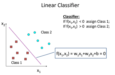
Let's have a look at Linear Classifier

Perceptron:-

• Perceptron is the name given to the linear classifier.
• If there exists a Perceptron that correctly classifies all the training examples, then we say that the training set is linearly separable.
• There are different Perceptron learning techniques are available.

Perceptron - Let's begin with linearly separable data:-

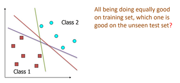
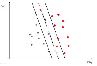
• For linearly separable data many Perceptrons are possible that correctly classifies the training set.
  

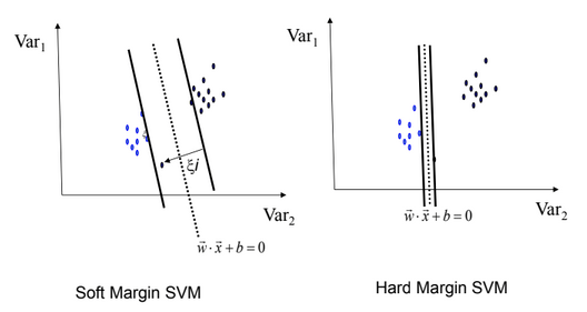
Hard-margin SVMs:-

The best perceptron for a linearly separable data is called "hard linear SVM"

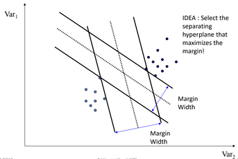
• For each linear function we can define its margin.
• That linear function which has the maximum margin is the best one.
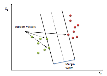
• Maximizing margin
  

Support Vectors:-

• The vectors (cases) that define the hyperplane are the support vectors.
  
• What if the data is not linearly separable?
  
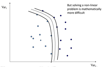
• So, there is a solution for that => kernel Trick.

Kernel-Trick:-

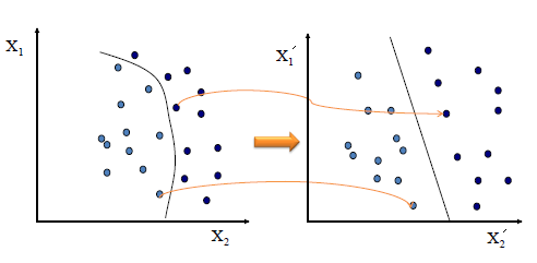
• Map data(Input-Space) to high dimensional space(known as Feature-Space) where it is easier to classify with linear decision surfaces: reformulate problem so that data is mapped implicitly to this(Input-Space) space.
  
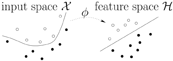
  See an example for that, how it's mapping to a higher dimension and converting to linearly separable data.
  
  Consequently, there is no need to do this mapping explicitly.

The Trick!!!:-

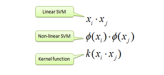
• For some mappings, the dot product in the feature space can be expressed as a function in the input space.
  $\phi \left ( X_1\right ).\phi \left ( X_2\right ) = k(X_1,X_2)$
  Eg:- Consider a two dimensional problem with
  $\mbox{If } X = \left ( x_1,x_2\right )^{t}. \mbox{ Let } \phi\left(x_1^2,x_2^2,\sqrt{2}x_1x_2\right)^t \nonumber \$
  Then, $\phi(X_i).\phi(X_j) = k(X_i,X_j) = (X_i.X_j)^2.$
  
• So, if the solution is going to involve only dot products then it can be solved using kernel trick(of course, appropriate kernel function has to be chosen).
• The problem is, with powerful kernels like "Gaussian kernel" it is possible to learn a non-linear classifier which does extremely well on the training set.
• Discriminant functions: non-linear:-
  
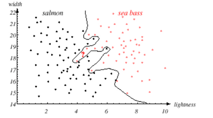
  • This makes zero mistakes with the training set.
• Other important issues...
  • This classifier is doing very well as for the training data is considered, but this does not guarantee that the classifier works well with a data element which is not there in the training set (that is, with unseen data).
  • This is overfitting the classifier with the training data.
  • Maybe we are respecting noise also (There might be mistakes while taking the measurements).
  • The ability "to perform better with unseen test patterns too" is called the generalization ability of the classifier.
  • Generalization ability:-
    • it's argued that the simple one will have better generalization ability.
    • How to quantify this?
    • (Training error + a measure of complexity) should be taken into account while designing the classifier.
    • Support vector machines are proved to have better generalization ability.
      
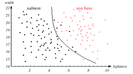
      -> This has some training error, but this is a relatively simple one.
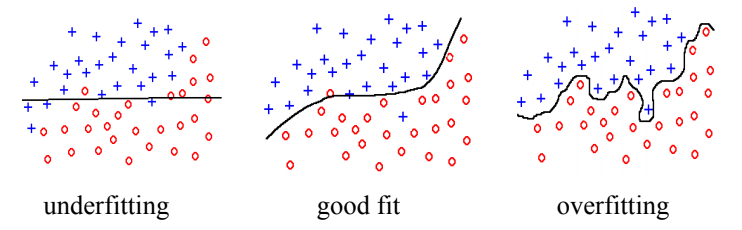
• Overfitting and underfitting revisited:-
  

Soft-margin SVMs:-

• It allows for some mistakes with the training set!
• But, this is to achieve a better margin.
  

So, Formally speaking about SVMs:-

• Decision surface is a hyperplane(line in 2D) in feature space(similar to the Perceptron).
• In a nutshell:
  • Map the data to a predetermined very high-dimensional space via a kernel function
  • Find the hyperplane that maximizes the margin between the two classes
  • If data are not separable find the hyperplane that maximizes the margin and minimizes the (penalty associated with) misclassifications.

Three key ideas:-

[1]. Define what an optimal hyperplane is (in a way that can be identified in a computationally efficient way): maximize margin <- Linear Hard-margin SVMs

[2]. Extend the above definition for non-linearly separable problems: have a penalty term for misclassifications <- Linear Soft-margin SVMs

[3]. Map data to high dimensional space where it is easier to classify with linear decision surfaces: reformulate problem so that data is mapped implicitly to this space <- Non-Linear Hard/Soft-margin SVMs

Let's look at it one by one...

[1] By Looking at Perceptron as we discussed earlier, can you tell me, Which Separating Hyperplane to Use?, the solution is Hard Linear SVM -> we need to maximizing the margin. So,how to maximize let's have a look with a little bit test of math.
Setting Up the Optimization Problem

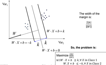
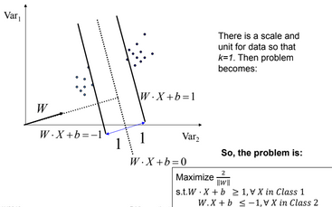
By taking intercept value K equal to one, we get distance(margin) between both support vectors as follows.

• If class-1 corresponds to 1 and class-2 corresponds to -1, we can re-write the problem
  $$ W.X_i + b \geq 1, \forall X_i ,\mbox{with } y_i = 1$$
  $$W.X_i + b \leq -1, \forall X_i ,\mbox{with } y_i = -1$$
  $$\mbox{as, } y_i\left (W.X_i + b\right ) \geq 1, \forall X_i$$

So the problem becomes:-
$\mbox{Maximize } \frac{2}{\left || W \right ||} , \mbox{ s.t. } y_i\left ( W.X_i + b\right ) \geq 1, \forall X_i$
$\mbox{or, } \mbox{Minimize } \frac{1}{2}\left || W \right ||^2, \mbox{ s.t. } y_i\left ( W.X_i + b\right ) \geq 1, \forall X_i $

• So, now the problem is to find W, b that solves
  $$ \mbox{Minimize } \frac{1}{2}\left || W \right ||^2, \mbox{ s.t. } y_i\left ( W.X_i + b\right ) \geq 1, \forall X_i $$
  for this objective function we will solve in next section by using Quadratic Programming.
• Since, problem is convex so, there is a unique global minimum value(when feasible).
• This problem becomes Non-solvable if the data is not linear seprable
• Quadratic Programming
  • Very efficient computationally with modern constraint optimization engines(handles thousands of constraints).

[2]Non-Linearly Separable Data:- However, perfect separation may not be possible, or it may result in a model with so many cases that the model does not classify correctly. In this situation, SVM finds the hyperplane that maximizes the margin and minimizes the misclassifications.

The algorithm tries to maintain the slack variable(xi) to zero while maximizing margin. However, it does not minimize the number of misclassifications (NP-complete problem) but the sum of distances from the margin hyperplanes.
And now the objective function and constraints become as follows

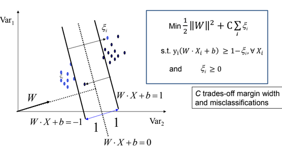
• As C --> ∞ We get closer to the Hard-margin SVMs.
• Parameter C can be viewed as a way to control over-fitting.

Robustness of Soft vs Hard Margin SVMs:-

Soft-Margin SVMs	Hard-Margin SVMs
Soft-Margin always have a solution	Not necessary always
Soft-Margin is more robust to outliers(Smoother surfaces (in the non-linear case)	But, can't do well in case of outliers
Need tuning of the parameter by using cross-validation	Hard-Margin does not require to guess the cost parameter (requires no parameters at all)

The simplest way([1] or [2]) to separate two groups of data is with a straight line(1 dimension), flat plane(2 dimensions) or an N-dimensional hyperplane. However, there are situations where a nonlinear region can separate the groups more efficiently.SVM handles this problem by using a kernel function[3] (nonlinear) to map the data into a different space where a hyperplane(linear) cannot be used to do the separation. It means a non-linear function is learned by a linear learning machine in a high dimensional feature-space while the capacity of the system is controlled by a parameter that does not depend on the dimensionality of the space.
This is called kernel-trick which means the kernel function transform the data into a higher dimensional feature space to make it possible to perform the linear separation.

So, that's why we go to 3rd key idea(which is universal)
[3] Mapping Data to High-Dimensional Space:-

• Find function $\Phi(x)$ to map to a different space, then SVM formulation becomes:
  (Hard-margin SVMs)
  $$ \mbox{min } \frac{1}{2}\left || W \right ||^2, \mbox{ s.t. } y_i\left ( W.\Phi(X) + b\right ) \geq 1, \forall X_i $$
  (Soft-margin SVMs)
  $$\mbox{min } \frac{1}{2}\left ||W\right ||^2 + C\sum_{i}\xi_{i}$$
  $$\mbox{subject to: }y_i(W.\Phi(X) + b) \geq 1-\xi_i, \forall X_i,\mbox{and } \xi_i \geq 0, \forall{i}$$

• Data appear as $\Phi(X)$, weights W are now weights in the new space

• Explicit mapping expensive if $\Phi(X)$ is very high dimensional

• Solving the problem without explicitly mapping the data is desirable

So, finally, it's time to solve these minimization problems of Objective functions with corresponding constraints, which we will discuss in the next section(3). --> Prerequisite
If you don't wanna know in-depth of SVMs formulation then directly move forward to section-4.

3. Mathematical explanation:-

Constrained optimization:-

In mathematical optimization, constrained optimization (in some contexts called constraint optimization) is the process of optimizing an objective function with respect to some variables in the presence of constraints on those variables. The objective function is either a cost function or energy function, which is to be minimized, or a reward function or utility function, which is to be maximized.

A general constrained optimization problem may be written as:-
$\mbox{min } f(v) $
$\mbox{subject to: } g_i(v) = c_i, \mbox{ for i=1,...,n } \mbox{ Equality constraints} $
$\mbox{ } h_j(v) \geq d_j, \mbox{for j=1,...,n } \mbox{ Inequality constraints}$
$\mbox{where, } g_i(v) = c_i \mbox{ for } i=1,...,n\mbox{ and } h_j(v) \geq d_j\mbox{ for } j=1,...,m$

Linear SVMs(Hard-margin):-

• The problem is(objective function):
  $$ \mbox{min } \frac{1}{2}||W||^2, \mbox{ subject to constraints. } 1 - y_i\left ( W.X_i + b\right ) \leq 0, \forall i $$
• Note that the objective function is convex and the constraints are linear. so Lagrangian method can be applied.

=> Lagrangian,
$$ L = f(v) + \sum_{j=1}^{n}\alpha _jg_j(v) $$
where $v$ is called primal variables and $\alpha_j$ are the lagrangian multipliers which are also called dual variables.

• $L$ has to be minimized with respect to primal variables and maximized with respect to dual variables.

• But what if more than one inequality constraints are there.

• So, there is a solution for that By using K.K.T.(Karush-Kuhn-Tuker) conditions we can come up with the the solution as follows:-

  • The K.K.T conditions "necessary" at optimal $v$ are:
  1. $\nabla_{v}L = 0$
  2. $\alpha_j \geq 0 \mbox{, for all j=1,...,n}$
  3. $\alpha_jg_j(v) = 0 \mbox{, for all j=1,...,n} $

  If $f(v)$ is convex and $g_j(v)$ is linear for all j, then it turns out that K.K.T conditions are "necessary and sufficient" for the optimal $v$.

• $$ \mbox{min } \frac{1}{2}\left || W \right ||^2, \mbox{ subject to constraints. } 1 - y_i\left ( W.X_i + b\right ) \leq 0, \forall i $$

• Our SVM objective function in the form form of Lagrangian is something like this,

  • $ L(W, b, i) = \frac{1}{2}\left ||W \right ||^2 + \sum_{i}\alpha_i[1 - y_i\left ( W.X_i + b\right)]$
    here, $\alpha = (\alpha_1 . . .\alpha_n)$
    By applying K.K.T conditions...
    
  • we solve these equations (1), (2), (3) and (4) to get $W$ and $b$.
  • While it is possible to do this, it is tedious.
    => Indeed, there is n another method called "Wolfe Dual Formation" by which we can solve or formulate the objective function easily.

• Other easy and advantageous ways to solve the optimization problem does exist which can be easily extended to non-linear SVMs.

• This is to get $L$ where we eliminate $W$ and $b$ which has $\alpha_1,...,\alpha_n$.

• We know, $L$ has to be maximized w.r.t the dual variables $\alpha_1,...,\alpha_n$.
  Now, the Lagrangian $L$ is:
  

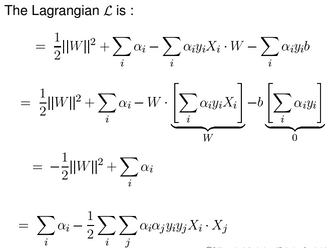
• so, our task is to Maximize $L$ w.r.t $\alpha$
  $$L = \sum_{i}\alpha_i - \frac{1}{2}\sum_{i}\sum_{j}\alpha_i\alpha_jy_iy_jX_i.X_j$$
  such that $\sum\alpha_iy_i = 0$ and $\alpha_i \geq 0$ for all $i$.

• We need to find the Lagrangian multipliers $\alpha_i(1 \leq i \leq n)$ only.

• Primal variables $W$ and $b$ are eliminated, that's great.

• There exists various numeric iterative methods to solve this constrained convex quadratic optimization problem.

• Sequential minimal optimization(SMO) is one such technique is a simple and relatively fast method.

• $\alpha = (\alpha_1,...,\alpha_n)$, let $1 = (1,...,1)^t$ then
  $$L = -\frac{1}{2}\alpha^t\hat{K}\alpha + 1^t\alpha $$
  where $\hat{K}$ is a $n x n$ matrix with its (i, j)th entry being $(y_iy_jX_i.X_j)$

• if $\alpha_i \geq 0$(from(4)) $\Rightarrow X_i$ is on a hyperplane, i.e., $X_i$ is a support vector.
  Note: $X_j$ lies on the hyperplane $ \neq> \alpha_i \geq 0$

• Similarly, $X_i$ doesn't lie in hyperplane $\Rightarrow \alpha_i = 0$
  That is, for interior points $\alpha_i = 0$.

so, the Solution would be:-

• Once $\alpha$ is known, We can find $W = \sum_i\alpha_iy_iX_i$
• The classifier is as follows:-
  $$f(X) = Sign(W.X + b) = Sign\begin{Bmatrix} \sum_{i}\alpha_iy_iX_i.X + b\end{Bmatrix}$$
• b can be found from (4)
  • For any $\alpha \neq 0$, we have $y_j(W.X_j + b) = 1$
  • By multiplying with y_j on both sides we get, $W.X_j + b = y_j$
  • So, $b = y_j - W.X_j = y_j - \sum_i\alpha_iy_iX_i.X_j$

=> We got some observations from the results...
- In the dual problem formulation and in its solution we have only dot products between some of the training patterns.
- Once we have the matrix $\hat{K}$, the problem and its solution are independent of the dimensionality $d$.

Non-linear SVMs:-

• We know that every non-linear function in $X$-space(input-space) can be seen as a linear function in an appropriate $Y$-space(feature space).
• Let the mapping be $Y = \phi(X)$.
• Once the $\phi(.)$ is defined, one has replace in the problem as well in the solution, .for the certain products, as explained below.
• Whenever we see $X_i.X_j$, replace this by $\phi(X_i).\phi(X_j)$.
• While it is possible to explicitly define the $\phi(.)$ and generate the training set in the $Y$-space, and then obtain the solution...
• It is tedious and amazingly unnecessary also.
  So, Indeed - Kernel trick comes in mind as we discussed in Kernel Trick section.

Soft-margin Formulation:-

• Until now, we assumed that the data is linearly (or non-linearly) separable.
• The SVM derived is sensitive to noise.
• Soft Margin formulation allows violation of the constraints to some extent. That is, we allow some of the boundary patterns to be misclassified.

As we earlier saw, In soft-margin formulation we introduce slack variables and Cas a penalty parameter
Now, the objective function to minimize is:
$$\mbox{min } \frac{1}{2}\left ||W\right ||^2 + C\sum_{i}\xi_{i}$$
$$\mbox{subject to: } 1-\xi_i - y_i(W.X + b) \leq 0, \forall X_i,\mbox{ and} \xi_i \geq 0 \forall i$$
$$\mbox{where } C \geq 0$$

• Note that the objective function is convex and the constraints are linear. so Lagrangian method can be applied.
  => Lagrangian on soft_margin SVMs as follows:-
  $$L = \frac{1}{2} ||W||^2 + C\sum_i\xi_i + \alpha_i[1-\xi_i - y_i(W.X + b)] - \sum\beta_i\xi_i$$
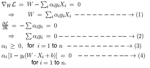
  By applying K.K.T Conditions...

1). $\nabla_{W}L = W - \sum\alpha_iy_iX_i = 0$
$\Rightarrow W = \sum\alpha_iy_iX_i \mbox{ } ---> (1)$

2). $\frac{\partial L}{\partial b} = -\sum\alpha_iy_i = 0$
$\Rightarrow \sum\alpha_iy_i = 0 \mbox{ } ---> (2)$

3). $\frac{\partial L}{\partial \xi_i} = C - \alpha_i - \beta_i = 0$
$\Rightarrow \alpha_i + \beta_i = 0 \mbox{ } ---> (3)$

4). $\alpha_i \geq 0 \mbox{ } ---> (4)$

5). $\beta_i \geq 0 \mbox{ } ---> (5)$

6). $\alpha_j(1-\xi_i - y_i(W.X + b)) = 0 \mbox{ } ---> (6)$

7). $\xi_i\beta_i = 0 \mbox{ } ---> (7)$

Same as before, this is tedious to solve all wquation with more variables, so again by using Wolfe Dual Formulation Indeed!!!.
Maximize $L$ w.r.t $\alpha$
$$L = \sum_i\alpha_i - \frac{1}{2}\sum_i\sum_j\alpha_i\alpha_jy_iy_jX_i.X_j$$
such that $\sum\alpha_iy_i = 0$, and $0 \leq \alpha_i \leq C, \forall i$

• where, $C = \infty \Rightarrow$ hard Margin
• and, $C = 0 \Rightarrow$ Very-Very Soft Margin

So, the training methods can we used as follows:-

• Any convex quadratic programming technique can be applied. But with larger training sets, most of the standard techniques can become very slow and space occupying. For example, many techniques needs to store the kernel matrix whose size is $n^2$ where $n$ is the number of training patterns.
• These considerations have driven the design of specific algorithms for SVMs that can exploit the sparseness of the solution, the convexity of the optimization problem, and the implicit mapping into feature space.
• One such a simple and fast method is Sequential Minimal Optimization (SMO).
  For understanding SVMs you can refer to this paper by Platt.

4. Implementation with python:-

In this section we will implement a real-world problem, SMS Spam classification by using SVM.
you can refer dataset here SMS Spam Collection Dataset. For details about dataset refer this kaggle dataset link.
For complete notebook refer here

Required Libraries:-

First of all import all required libraries.

import numpy as np
import pandas as pd
import matplotlib.pyplot as plt
from collections import Counter
from sklearn import feature_extraction, model_selection, metrics, svm

from IPython.display import Image
import warnings
warnings.filterwarnings("ignore")
%matplotlib inline

EDA:-

Observe the dataset in tabular format.

data = pd.read_csv('https://gist.githubusercontent.com/rajvijen/51255cf4875372b904bdb812a3b85b28/raw/816dcd4cdc7553faea396186067e814487046c74/sms_spam_classification_data.csv', encoding='latin-1')
data.head(10)

Output: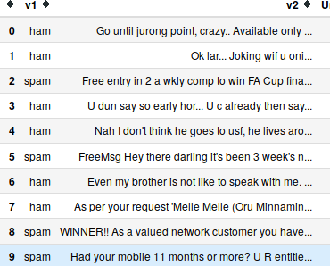

Get some insights from data.
Data Visualization:-

count_class = pd.value_counts(data["v1"], sort = True)
count_class.plot(kind = 'bar', color = ['blue', 'orange'])
plt.title('Spam vs Non-spam distribution of data')
plt.show()

Output: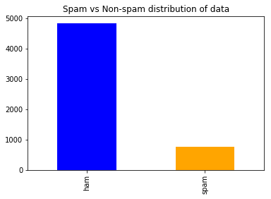

count_class.plot(kind = 'pie', autopct = '% 1.0f%%')
plt.title('Percentage distribution of data')
plt.ylabel('')
plt.show()

Output: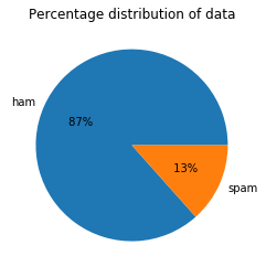

we need to know a little bit more about text data
Text Analytics:-
let's look at frequencies of words in spam and non-spam(ham) messages and plot that out.

count1 = Counter(" ".join(data[data['v1']=='ham']["v2"]).split()).most_common(20)
df1 = pd.DataFrame.from_dict(count1)
df1 = df1.rename(columns = {0: "non-spam words", 1 : "count"})

count2 = Counter(" ".join(data[data['v1']=='spam']["v2"]).split()).most_common(20)
df2 = pd.DataFrame.from_dict(count2)
df2 = df2.rename(columns={0: "spam words", 1 : "count_"})

Plots:-

df1.plot.bar(legend = False, color = 'green')
y_pos = np.arange(len(df1["non-spam words"]))
plt.xticks(y_pos, df1["non-spam words"])
plt.title('More frequent words in non-spam messages')
plt.xlabel('words')
plt.ylabel('number')
plt.show()

Output: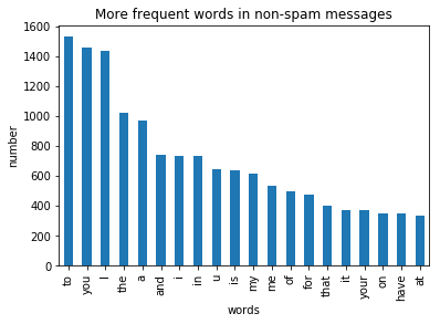

and for words in spam messages

df2.plot.bar(legend = False, color = 'red')
y_pos = np.arange(len(df2["spam words"]))
plt.xticks(y_pos, df2["spam words"])
plt.title('More frequent words in spam messages')
plt.xlabel('words')
plt.ylabel('number')
plt.show()

Output: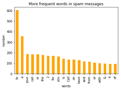
By visualizing and observation we can say that most of frequest words in both classes are stop words such as 'to', 'a', 'or'.
For better accuracy in the model, it's better to remove stop words.

Feature Engineering:-
The features in our data are important to the predictive models we use and will influence the results we are going to achieve. The quality and quantity of the features will have great influence on whether the model is good or not.
so, first or most remove stop words.

f = feature_extraction.text.CountVectorizer(stop_words = 'english')
X = f.fit_transform(data["v2"])
np.shape(X)

Output: (5572, 8409)

So, finally, our goal is to detect spam words.
Predictive Modelling:-

First of all transform the categorical variables(spam/non-spam) into binary variable(1/0) by using label encoding.

data["v1"] = data["v1"].map({'spam:1','ham':0})

Now, split the data into train and test set.

X_train, X_test, y_train, y_test = model_selection.train_test_split(X, data['v1'], test_size=0.33, random_state=42)
print([np.shape(X_train), np.shape(X_test)])

Output: [(3733, 8409), (1839, 8409)]

So, now use sci-kit learn's in-built SVC(support vector classifier) with Gaussian kernel for predictive modelling.
We train the model by tuning regularization parameter C, and evaluate the accuracy, recall and precision of the model with the test set.

# make a list of parameter's to tune for training
list_C = np.arange(500, 2000, 100)  #100000
# zeros initialization
score_train = np.zeros(len(list_C))
score_test = np.zeros(len(list_C))
recall_test = np.zeros(len(list_C))
precision_test= np.zeros(len(list_C))

count = 0
for C in list_C:
    # Create a classifier: a support vector classifier
    clf = svm.SVC(C = C, kernel=’rbf’, degree=3, gamma=’auto_deprecated’)
    
    # learn the texts
    clf.fit(X_train, y_train)
    score_train[count] = clf.score(X_train, y_train)
    score_test[count]= clf.score(X_test, y_test)
    recall_test[count] = metrics.recall_score(y_test, clf.predict(X_test))
    precision_test[count] = metrics.precision_score(y_test, clf.predict(X_test))
    count = count + 1 

Acuraccy metrices

Let's look at accuracy metrics with parameter C.

matrix = np.matrix(np.c_[list_C, score_train, score_test, recall_test, precision_test])
models = pd.DataFrame(data = matrix, columns = 
             ['C', 'Train Accuracy', 'Test Accuracy', 'Test Recall', 'Test Precision'])
models.head(10)

Output: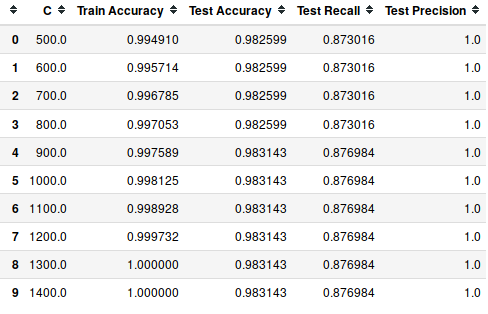

Check the model with the most test precision.

best_index = models['Test Precision'].idxmax()
models.iloc[best_index, :]

Output:

    C                 500.000000
    Train Accuracy      0.994910
    Test Accuracy       0.982599
    Test Recall         0.873016
    Test Precision      1.000000
    Name: 0, dtype: float64

This model doesn't produce any false-positive, which is expected.
Let's check if there is more than one model with 100% precision.

models[models['Test Precision']==1].head(5)

Output:

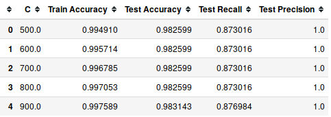
Among these models with the highest possible precision, we are going to select which has more test accuracy.

best_index = models[models['Test Precision']==1]['Test Accuracy'].idxmax()

# check with the best parameter(C) value 
clf = svm.SVC(C=list_C[best_index])
clf.fit(X_train, y_train)
models.iloc[best_index, :]

Output:
    C                 900.000000
    Train Accuracy      0.997589
    Test Accuracy       0.983143
    Test Recall         0.876984
    Test Precision      1.000000
    Name: 4, dtype: float64

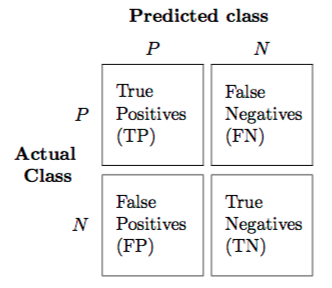
Confusion matrix:-

confusion_metrix_test = metrics.confusion_metrix(y_test, clf.predict(X_test))
pd.DataFrame(data = confusion_metrix_test, columns = ['Predicted 0', 'Predicted 1'], index = ['Actual 0', 'Actual 1'])

Output: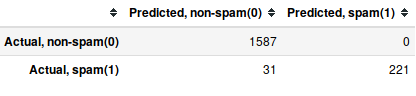

We misclassify 31 spam messages as non-spam messages whereas we don't misclassify any non-spam message.

Results:-

We got 98.3143% accuracy, which is quite well with SVM classifier.

It classifies every non-spam message correctly (Model precision)

It classifies the 87.7% of spam messages correctly (Model recall)

5. Applications of SVMs in the real world:-

1. Face detection
2. Text and hypertext categorization
3. Classification of images
4. Bio-informatics(cancer classification)
5. Protein fold and remote homology detection
6. Handwriting Recognition
7. Generalized predictive control(GPC) etc.

I hope you enjoyed the complete journey of SVMs, If you have any query or idea, please post in the comment section below.