
Open-Source Internship opportunity by OpenGenus for programmers. Apply now.
Zipf's Law is an empirical law, that was proposed by George Kingsley Zipf, an American Linguist.
According to Zipf's law, the frequency of a given word is dependent on the inverse of it's rank . Zipf's law is one of the many important laws that plays a significant part in natural language processing, the other being Heaps' Law.
f(r, α) ∝ 1⁄rα
Here,
- α ≈ 1
- r = rank of a word
- f(r, α) = frequency in the corpus
The word with the second highest rank will have the frequency value ½ of the first word, the word with the third highest rank will have the frequency value ⅓ of the first word, and so on...
Some points to note about Zipf's Law
If we consider a constant for the following law, we have:
f = k⁄rα
=> f × rα = k
=> f × r = k
This constant would be same for every word in expected results, but that is not the case for observed result. This will be further shown in the sample code, and explained later, but just remember this for now - few of the highest and the lowest words will not have the same values of k - only the data in the middle range of ranks follow this - and this is only for our particular document. There are other variants of Zip's law, like Zipf-Mandelbrot law, that tries to fit the frequencies, by adding an offest β, and it is given by:
f(r, α, β) ∝ 1⁄(r+β)α
Here, β ≈ 2.7, and it is also known as the rank offset.
Note:
Values of α and β cannot be always taken as equal to 1 and 2.7 - they are parameters that can be tuned to fit a data perfectly, and there are cases where you may have to adjust the value, if the results are not satisfactory.
Fun fact about Zipf's law
Zipf's law is an empirical law, that models the frequency distribution of words in languages. And by languages, this is not just restricted to English corpora. In fact, it was even found out that the language spoken by dolphins, which are a given set of whistles and high frequency shrills, also follow Zipf's Law!
Terminologies
- Frequency - Frequency is the number of occurences of a word in the given document or corpus.
- Rank - The rank of a word can be defined as the position occupied, for having the highest number of occurence in the given document or corpus. A word with the highest frequency will have the highest rank.
- Document - A piece of printed, written, or electronically stored material that can transmit information or evidence. Latin for Documentum, which denotes a "teaching" or "lesson".
- Corpus - A collection of texts, or written information (known as documents), usually about the works of a particular author, or a given subject/ topic. Usually stored as electronic format.
Program on Zipf's law
First, we start with importing the required libraries. NLTK is actually where we will be accessing our corpus from.These documents are available at "C:\Users\ashvi\AppData\Roaming\nltk_data\corpora\gutenberg", in Windows.
For this particular code, I will be using "carroll-alice.txt". You may have to download them before.
# %% Import libraries required
from operator import itemgetter
import nltk
import pandas as pd
from nltk.corpus import stopwords
from matplotlib import pyplot as plt
Then we start by adding required variables, like frequency (frequency), word in the document (words_doc) and stopwords (stop_words). It removes symbols like '.', '?'and also articles like 'the', 'an', just to show a few.
# %% Initialize frequency, and import all the words in a corpus
frequency = {}
words_doc = nltk.Text(nltk.corpus.gutenberg.words('carroll-alice.txt'))
stop_words = set(stopwords.words('english'))
Next, we convert all the letters to lower cases, by the following code.
# %% Convert to lower case and remove stop words
words_doc = [word.lower() for word in words_doc if word.isalpha()]
words_doc = [word for word in words_doc if word not in stop_words]
The for-loop will calculate the frequency of the words inside - it creates a dictionary data type of the form {'word' : number}. We also create a DataFrame (df) which is part of the Pandas (pd) library, followed by initializing basic variables like rank, and column_header.
You can also see the collection variable, which will sort the given dictionary frequency.The next part is for printing the table, in ordered fashion.
# %% Calculate the frequency of the words inside
for word in words_doc :
    count = frequency.get(word , 0)
    frequency[ word ] = count + 1

rank = 1
column_header = ['Rank', 'Frequency', 'Frequency * Rank']
df = pd.DataFrame( columns = column_header )
collection = sorted(frequency.items(), key=itemgetter(1), reverse = True)
Here, we finally print our dataframe to the console
Warning!
This is a very machine intensive task, and if performed on an older device, could take some time.
# %%Creating a table for frequency * rank

for word , freq in collection:
    df.loc[word] = [rank, freq, rank*freq]
    rank = rank + 1

print (df)
But this is far from over! Since numbers are not great for visualization, we need to find a better way to show our values. This is what we get as our output in our console, if we execute all the code.
       Rank Frequency Frequency * Rank
to        1      5239             5239
the       2      5201            10402
and       3      4896            14688
of        4      4291            17164
i         5      3178            15890
    ...       ...              ...
true    296        66            19536
heart   297        66            19602
talked  298        66            19668
sir     299        66            19734
ready   300        66            19800

[300 rows x 3 columns]
We will be using one of the most useful tools available in Python - pyplot, provided by the matplotlib library. We chose to use bar graph to represent our values, as it is the perfect way to represent frequencies with respect to words.
# %% Python visualization with pyplot
plt.figure(figsize=(20,20))  #to increase the plot resolution
plt.ylabel("Frequency")
plt.xlabel("Words")
plt.xticks(rotation=90)    #to rotate x-axis values

for word , freq in collection[:30]:
    plt.bar(word, freq)
plt.show()
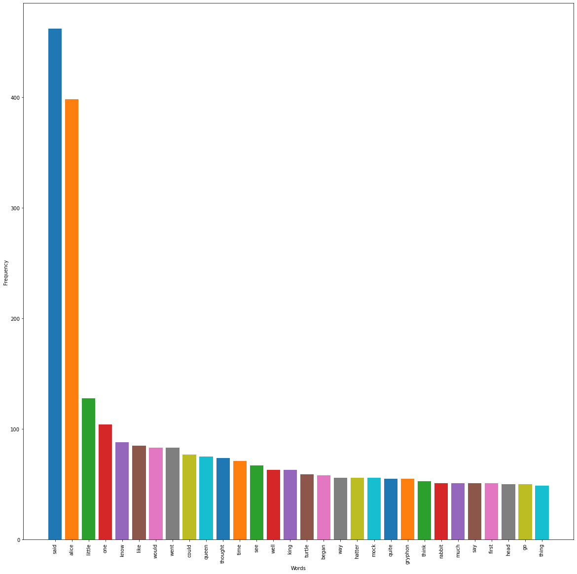
This is how our visualized data looks like! From this, you can understand that our second word 'alice' is 1⁄2α times the first word 'said'. The third word 'little' is 1⁄3α; the frequency of the word 'said'. And so, the rest of the frequency keeps getting shorter in the series of 1⁄4α, 1⁄5α, 1⁄6α....
So, overall, our Python program should look something like this
# %% Import libraries required
from operator import itemgetter
import nltk
import pandas as pd
from nltk.corpus import stopwords
from matplotlib import pyplot as plt

# %% Initialize frequency, and import all the words in a corpus
frequency = {}
words_doc = nltk.Text(nltk.corpus.gutenberg.words('carroll-alice.txt'))
stop_words = set(stopwords.words('english'))

# %% Convert to lower case and remove stop words
words_doc = [word.lower() for word in words_doc if word.isalpha()]
words_doc = [word for word in words_doc if word not in stop_words]

# %% Calculate the frequency of the words inside
for word in words_doc :
    count = frequency.get(word , 0)
    frequency[ word ] = count + 1

rank = 1
column_header = ['Rank', 'Frequency', 'Frequency * Rank']
df = pd.DataFrame( columns = column_header )
collection = sorted(frequency.items(), key=itemgetter(1), reverse = True)

# %%Creating a table for frequency * rank

for word , freq in collection:
    df.loc[word] = [rank, freq, rank*freq]
    rank = rank + 1

print (df)

# %% Python visualization with pyplot
plt.figure(figsize=(20,20))  #to increase the plot resolution
plt.ylabel("Frequency")
plt.xlabel("Words")
plt.xticks(rotation=90)    #to rotate x-axis values

for word , freq in collection[:30]:
    plt.bar(word, freq)
plt.show()
# %% End of the program
Significance of k, the constant
The value that we discussed earlier seems to have no relationship with both the dataframe, as well as the visualization. This is because of the fact that there were too many words to fit inside the chart, and the console would truncate automatically.
So, how do we prove that? Spyder IDE has a feature, called the Variable Explorer, from which we can visualize all the possible variables, and we will put that to test.
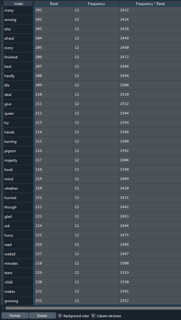
As said before, the value of k is not valid for the first and the last few data in our example, which will be explained further below, and so, we will choose some random values from between.
Screenshot 1:
Screenshot 2:
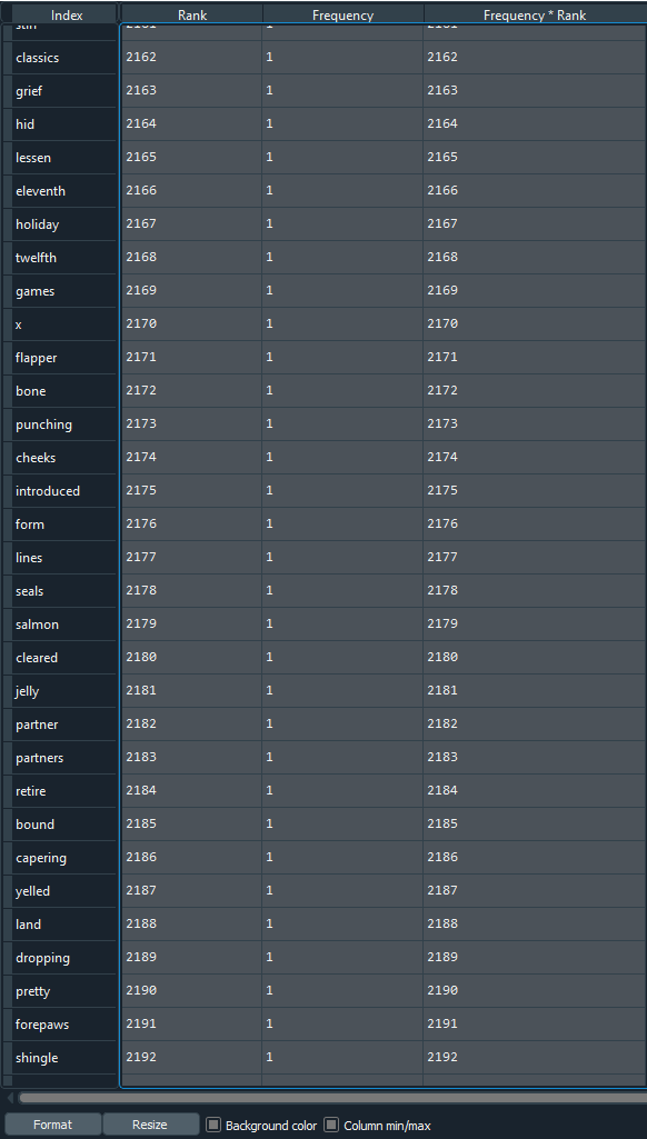
We can see that both the screenshots have a large gap in their ranks, but they are values from somewhere in the middle.If you check the value of 'Frequency * Rank' (which is k), you can see that most of the values are nearly similar, especially within a screenshot. So the laws do hold true for words.
Python files for reference:
To access the files, please click on the following link:
https://github.com/Ashvith/Zipf-s-Law
It contains both .py, as well as .ipynb format.
Problems with Zipf's law
Zipf's law require that the size of the material that is to be worked on, should be as large as a mature corpus - and not just from a source or two. The deviations in our first and last few terms were because of the simple reason that we used a simple document with a word count of 26,443 - this isn't sufficient to begin with. For more accurate results, you could use Brown Corpus (nearly 6 million words), Gutenberg or Google Book's corpus (155 million words for American English)- although it could take a lot of time processing, and you may need to move to Google's Colaboratory, or other such platforms.
Note:
You could use the whole Gutenberg corpus, by changing this code snippet:words_doc = nltk.Text(nltk.corpus.gutenberg.words('carroll-alice.txt'))to this one:
words_doc = nltk.Text(nltk.corpus.gutenberg.words())or for Brown corpus:
words_doc = nltk.Text(nltk.corpus.brown.words())
Question 1
What is the importance of Zipf's law in data science and machine learning?
Question 2
Is there any specific requirement for Zipf's Law?
Question 3
What is significant about the value of k in expected outcome?
<center>f = <sup><i>k</i></sup>⁄<sub>r<sup>α</sup></sub></center>
<center>=> f × r<sup>α</sup> = <i>k</i></center>
<center>=> f × r = <i>k</i></center>
<center><b>(Since α is nearly equal to 1, we can ignore it for this case)</b></center>
This means that for the given word, we can have a value of f and r, which would give us the same value of <i>k</i>.
Sources
- Video on Zipf's law (video) by Victor Lavrenko
- Zipf's law as universal law for all language (video) by NOVA PBS official.