Basics of Quantization in Machine Learning (ML) for Beginners

Quantization in Machine Learning (ML) is the process of converting data in FP32 (floating point 32 bits) to a smaller precision like INT8 (Integer 8 bit) and perform all critical operations like Convolution in INT8 and at the end, convert the lower precision output to higher precision in FP32.
This sounds simple but as you can imagine that converting a floating point to integer results in error that can grow up through calculations, maintaining the accuracy is critical. In Quantization, accuracy is within 1% of the original accuracy.
In terms of performance, as we are dealing with 8 bits instead of 32 bits, we should be theretically 4 times faster. In real life applications, speedup of at least 2X is observed.
In this article, we will go through the basics of Quantization in Machine Learning quickly. Once you go through this article, you will be able to answer:
- How accuracy is recovered in Quantization?
- How doing calculation in INT8 or FP32 gives the same result?
The main topics in Quantization which we have covered in depth are:
- Lower precision
- Quantization fundamentals
- Range mapping
- Affine Quantization
- Scale Quantization
- Quantization granularity
- Calibration
- Post Training Quantization
- Weight Quantization
- Activation Quantization
- Recover Accuracy in Quantization
- Partial Quantization
- Quantization Aware Training
- Learning Quantization Parameters
- Overall Quantization process
Lower precision
The lower precision data type can be anything like:
- FP32
- FP16
- INT32
- INT16
- INT8
- INT4
- INT1
As per the current state of research, we are struggling to maintain accuracy with INT4 and INT1 and the performance improvement with INT32 oe FP16 is not significant.
The most popular choice is: INT8
When we are doing calculations in a particular datatype (say INT8), we need another structure with a datatype which can hold the result such that it handles overflow. This is known as accumulation data type. For, FP32, accumulation is FP32 but for INT8, accumulation is INT32.
This table gives you the idea of the reduction in data size and increase of mathematical power depending on the data type:
| Data type | Accumulation | Math Power | Data size reduced |
|---|---|---|---|
| FP32 | FP32 | 1X | 1X |
| FP16 | FP16 | 8X | 2X |
| INT4 | INT32 | 16X | 4X |
| INT4 | INT32 | 32X | 8X |
| INT1 | INT32 | 128X | 32X |
Quantization fundamentals
There are two basic operations in Quantization:
- Quantize: Convert data to lower precision like INT8
- Dequantize: Convert data to higher precision like FP32
In general, Quantize is the starting operation while Dequantize is the last operation in the process.
Range mapping
INT8 can store values from -128 to 127. In general, an B bit Integer can have the range as -(2^B) to (2^B-1).
In Range mapping, we have to convert a data of range [A1, A2] to the range of the B bit Integer (INT8 in our case).
Hence, the problem is to map all elements in the range [A1, A2] to the range [-(2^B), (2^B-1)]. Elements outside the range of [A1, A2] will be clipped to the nearest bound.
There are two main types of Range mapping in Quantization:
- Affine quantization
- Scale quantization
For quantization, there are two main types of mapping equation that are used by the above techniques:
F(x) = s.x + z
where, s, x and z are real numbers.
The special case of the equation is:
F(x) = s.x
s is the scale factor and z is the zero point.
Affine Quantization
In Affine Quantization, the parameters s and z are as follows:
s = (2^B + 1)/(A1-A2)

z = -(ROUND(A2 * s)) - 2^(B-1)
For INT8, s and z are as follows:
s = (255)/(A1-A2)

z = -(ROUND(A2 * s)) - 128
Once you convert all the input data using the above equation, we will get a quantized data. In this data, some values may be out of range. To bring it into range, we need another operation "Clip" to map all data outside the range to come within the range.
The Clip operation is as follows:
clip(x, l, u) = x   ... if x is within [l, u]

clip(x, l, u) = l   ... if x < l

clip(x, l, u) = u   ... if x > u
In the above equation, l is the lower limit in the quantization range while u is the upper limit in the quantization range.
So, the overall equation for Quantization in Affine Quantization is:
x_quantize = quantize(x, b, s, z)

    = clip(round(s * x + z),
           −2^(B−1),
           2^(B−1) − 1)
For dequantization, the equation in Affine Quantization is:
x_dequantize = dequantize(x_quantize, s, z) = (x_quantize − z) / s
Scale Quantization
The difference in Scale Quantization (in comparison to Affine Quantization) is that in this case, the zero point (z) is set to 0 and does not play a role in the equations. We use the scale factor (s) in the calculations of Scale Quantization.
We use the following equation:
F(x) = s.x
There are many variants of Scale Quantization and the simpliest is Symmetric Quantization. In this, the resultant range is symmetric. For INT8, the range will be [-127, 127]. Note that we are not considering -128 in the calculations.
Hence, in this, we will quantize a data from range [-A1, A1] to [-(2^(B-1), 2^(B-1)]. The equations for Quantization will be:
s = (2^(B - 1) − 1) / A1
Note, s is the scale factor.
The overall equation is:
x_quantize = quantize(x, B, s)
           = clip(round(s * x),
                  −2^(B - 1) + 1,
                  2^(B - 1) − 1)
The equation for dequantization will be:
x_dequantize = dequantize(x_quantize, s)
      = x_quantize / s
Quantization granularity
The input data is multi-dimensional and to quantize it, we can use the same scale value and zero point for the entire data or these parameters can be different for each 1D data in each dimension or different for each dimension.
This process of grouping the data for the quantization and dequantization process is known as Quantization Granularity.
The common choice of Quantization Granularity are:
- Per channel for 3D input
- Per row or Per column for 2D input
Hence, the scale value for a specific data like 3D input will be a vector of scale values where the i-th value will be the scale value for the i-th channel of the 3D input.
Choosing the granularity correctly helps in better representation of the data and accuracy at minimum cost of extra scale factors.
Calibration
Calibration in Quantization is the process of calculating the range [A1, A2] for the input data like weights and activations. There are three main methods of Calibration:
- Max
- Entropy
- Percentile
Max: This is the most simple method where we actually compare the input values to get the maximum and minimum value for the range A1 and A2.
Entropy: Use the KL Divergence method to choose A1 and A2 which minimizes the error between the orignal floating point data and the quantized data
Percentile: Consider only a specific percentage of values for calculation of the range and ignore the remaining percentage of large values which can be outliers. The ignored values are handled during clipping operation.
Post Training Quantization
Post Training Quantization is the process of quantizing available data like weights during training and embed it into the pre-trained model. There are two types of Post Training Quantization:
- Weight Quantization
- Activation Quantization
Weight Quantization
As the weights in a ML model does not depend on input, it can be quantized during training. Whe Batch normalization is used, we need to do per channel quantization or else the loss in accuracy is significant.
Hence, for weights, the most common choice is Max Calibration Per channel Quantization.
Activation Quantization
Max Calibration does work well with activation quantization but it is model specific. For some models like InceptionV4 and MobileNet variants, the drop in accuracy is significant (more than 1%).
For Activation Quantization, the best results are with 99.99% or 99.999% percentile calibration. The exact percentile value depends on the model.
Recover Accuracy in Quantization
The main challenge in Quantization is to maintain the accuracy and not less the accuracy fall by more than 1% as compared to FP32 inference process.
There are many ML models where the loss in accuracy is significant when Quantization is done. In this case, there are a couple of techniques that can be employed to bring back the accuracy during Quantization:
- Partial Quantization
- Quantization Aware Training
- Learning Quantization Parameters
Partial Quantization
In Partial Quantization, the idea is to do Quantization only for a few layers in a specific Machine Learning model and leave out the other layers.
We leave out the layers for which the loss in accuracy is maximum and is hard to maintain accuracy using the other techniques we explored. For these layer, FP32 inference is done. One example where Partial Quantization is used is BERT.
Quantization Aware Training
In Quantization Aware Training, the idea is to insert fake quantization operations within a graph before training and use this during fine-tuning the graph. The advantage is that when the model is training and the weights are calculated, the quantization factor plays a role in optimization function.
This techniques improves accuracy for almost all models except ResNeXt101, Mask RCNN and GNMT. This is because fine-tuning does not impact the accuracy beyond run to run variations.
Learning Quantization Parameters
The idea in Learning Quantization Parameters is to find the values for Quantization parameters like scale value, zero point, range value and others during the training of the model when the weights are calculated.
This produces good accuracy with most models as the Quantization parameters are associated with the weights.
Overall Quantization process
The overall Quantization process is as follows:
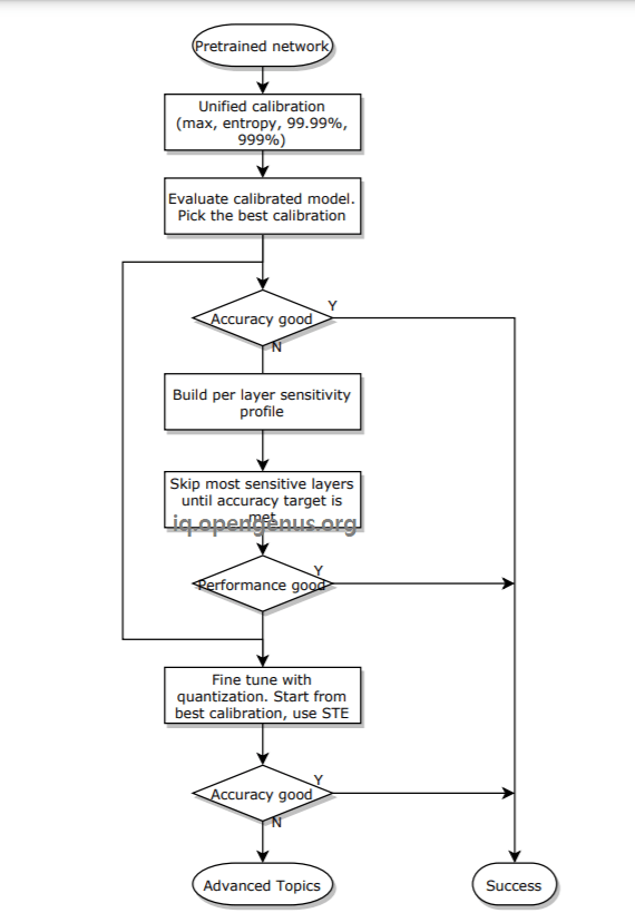
Hence, you are use Quantization on a pre-trained graph where weights are in quantized form. The knowledge of quantization (as covered in this OPENGENUS article) is useful to convert the FP32 input into quantized format and then, operated the operation like Convolution or ReLU as usually and quantize the output again as the resultant data may not be the quantized format.
With this, you have a strong understanding of Quantization in Machine Learning. This is the future read all our Quantization posts to stay updated in this fast moving area of research.