In this article, we have explained the idea and mathematics behind Contractive Autoencoders and the link with denoising autoencoder. We have presented a sample Python implementation of Contractive Autoencoders as well.

Table of content:

1. Introduction to Contractive autoencoder
2. Link between denoising and contractive autoencoder
3. Mathematics of Contractive autoencoder
4. Implementation of Contractive autoencoder

Terms to Know before learning about Contractive Autoencoders:

1. Frobenius norm
2. Jacobian Matrix
3. Sigmoid

Let us get started with Contractive Autoencoders.

Introduction to Contractive autoencoder

Contractive autoencoder is an unsupervised deep learning technique that helps a neural network encode unlabeled training data.

A simple autoencoder is used to compress information of the given data while keeping the reconstruction cost as low as possible. Contractive autoencoder simply targets to learn invariant representations to unimportant transformations for the given data.

It only learns those transformations that are provided in the given dataset so it makes the encoding process less sensitive to small variations in its training dataset.

The goal of Contractive Autoencoder is to reduce the representation’s sensitivity towards the training input data. In order to achieve this, we must add a regularizer or penalty term to the cost function that the autoencoder is trying to minimize.

So from the mathematical point of view, it gives the effect of contraction by adding an additional term to reconstruction cost and this term needs to comply with the Frobenius norm of the Jacobian matrix to be applicable for the encoder activation sequence.

If this value is zero, it means that as we change input values, we don't observe any change on the learned hidden representations.

But if the value is very large, then the learned representation is unstable as the input values change.

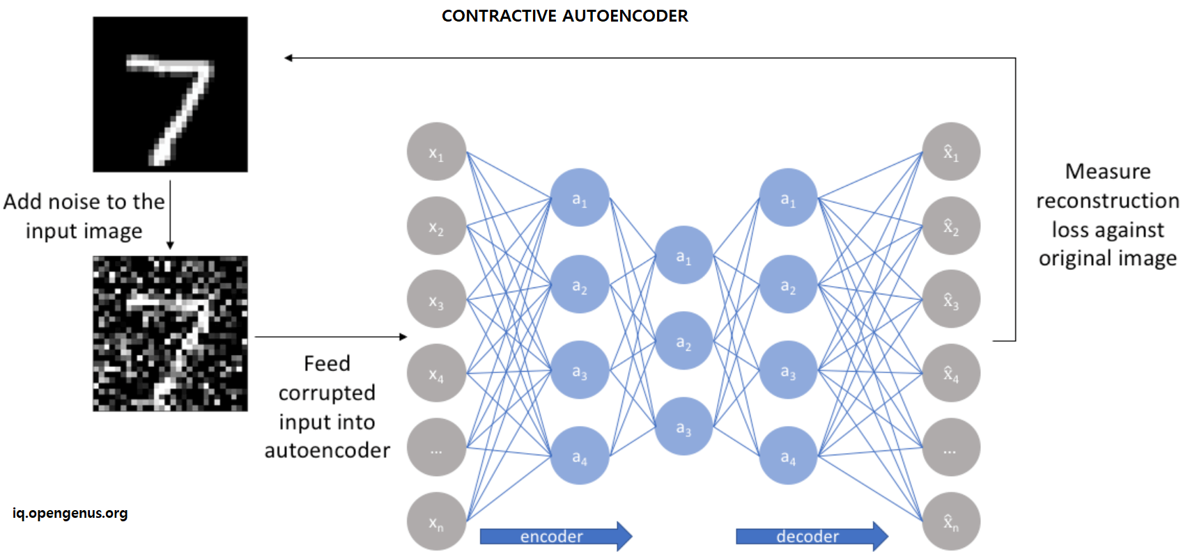
Contractive autoencoders are usually deployed as just one of several other autoencoder nodes, activating only when other encoding schemes fail to label a data point.

Link between denoising and contractive autoencoder

There is a connection between the denoising autoencoder and the contractive autoencoder:

the denoising reconstruction error is equivalent to a contractive penalty on the reconstruction function that maps x to r - g(f(x)).

In other words, denoising autoencoders make the reconstruction function resist small but finite sized perturbations of the input, whereas contractive autoencoders make the feature extraction function resist infinitesimal perturbations of the input.

When using the Jacobian based contractive penalty to pretrain features f(x) for use with a classifier, the best classification accuracy usually results from applying the contractive penalty to f(x) rather than to g(f(x)).

Mathematics of Contractive autoencoder

There are some important equations we need to know first before deriving contractive autoencoder. Before going there, we'll touch base on the Frobenius norm of the Jacobian matrix.

The Frobenius norm, also called the Euclidean norm, is matrix norm of an mxn matrix A defined as the square root of the sum of the absolute squares of its elements.

The Jacobian matrix is the matrix of all first-order partial derivatives of a vector-valued function. So when the matrix is a square matrix, both the matrix and its determinant are referred to as the Jacobian.

Combining these two defintions gives us the meaning of Frobenius norm of the Jacobian matrix.

The loss function is:

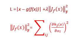
where the penalty term, λ(J(x))^2, is the squared Frobenius norm of the Jacobian matrix of partial derivatives associated with the encoder function and is defined in the second line.

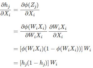
Now calculate the Jacobian of the hidden layer of our autoencoder. Assume that:

where ф is sigmoid nonlinearity. To get the j-th hidden unit, we need to get the dot product of the i-th feature and the corresponding weight. Then using chain rule and substituting our above assumptions for Z and h we get:

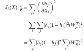
Our main objective is to calculate the norm, so we could simplify that in our implementation so that we don’t need to construct the diagonal matrix:

Implementation of Contractive autoencoder

Below are the steps of the formula and how they can be used in code to derive the contractive autoencoder.

Import all the libraries that we will need, namely numpy and keras.

import numpy as np
from keras.layers import Input, Dense
from keras.models import Model
import keras.backend as K

Use a small batch of 32 and 64 hidden units

X = np.random.randn(32, 786)
W = np.random.randn(786, 64)
Z = np.dot(W, X) #Z = W * X
h = sigmoid(Z) #taking sigmoid function of z

Here we find the derivative of h and the jacobian norm for each data point

Wj_sqr = np.sum(W.T**2, axis=1) 
dhj_sqr = (h * (1 - h))**2 
J_norm = np.sum(dhj_sqr)

These lines take the input from the user

inputs = Input(shape=(N,))
encoded = Dense(N_hidden, activation='sigmoid', name='encoded')(inputs)
outputs = Dense(N, activation='linear')(encoded)
model = Model(input=inputs, output=outputs)

In this method we calculate loss function using the last formula

def contractive_loss(y_pred, y_true):
    mse = K.mean(K.square(y_true - y_pred), axis=1)
    W = K.variable(value=model.get_layer('encoded').get_weights()[0])  
    W = K.transpose(W)
    h = model.get_layer('encoded').output
    dh = h * (1 - h)
    contractive = lam * K.sum(dh**2 * K.sum(W**2, axis=1), axis=1) #uses the last formula
    return mse + contractive #returns total loss calculated

model.compile(optimizer='adam', loss=contractive_loss) #creates a model of the autoencoder
model.fit(X, X, batch_size=N_batch, nb_epoch=5)

This completes the implementation of Contractive Autoencoders.

With this article at OpenGenus, you must have the complete idea of Contractive Autoencoders. Enjoy.