In this article, we have presented how Autoencoders can be used to perform Dimensional Reduction and compared the use of Autoencoder with Principal Component Analysis (PCA). We have provided a step by step Python implementation of Dimensional Reduction using Autoencoders.

Table of content:

1. Dimension Reduction with PCA and Autoencoders
2. Implementation of Dimensional reduction using autoencoder
3. Differences between PCA and autoencoder

Let us get started now.

Dimension Reduction with PCA and Autoencoders

There are a couple of ways to reduce the dimensions of large data sets like backwards selection, removing variables exhibiting high correlation, high number of missing values and principal components analysis to ensure computational efficiency. A relatively new method of dimensional reduction is by the usage of autoencoder.

Autoencoders are a branch of neural networks which basically compresses the information of the input variables into a reduced dimensional space and then it recreate the input data set to train it all over again.

Generally, the autoencoder is trained over a large number of iterations using gradient descent which effectively minimizes the mean squared error. T

he key component here is the bottleneck hidden layer. It is in this layer where the information from the input data has been compressed. So by extracting this layer from the model, each node can now be treated as a variable in the same way each chosen principal component is used as a variable in following models.

Principal components analysis is a method which reduces dimensionality of data by transforming the dataset into a set of principal components.

The first principal component explains the most amount of the variation in the data in a single component while the second one explains the second most amount of the variation, and so forth.

So if we choose the top k principal components that explain a significant amount of the variation, the other components can be dropped since they do not benefit the model as much as needed.

This procedure retains some of the latent information in the principal components which can help to build better models.

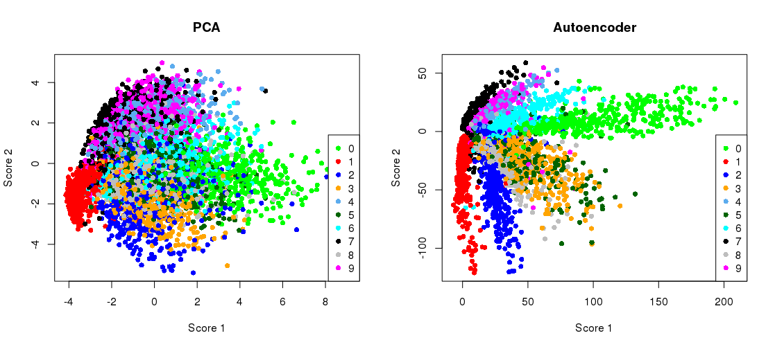
The below graph compares the amount of variation of reduction between PCA and autoencoders:

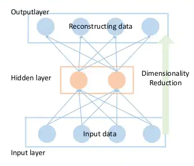
The architecture of an Autoencoder is as follows:

Implementation of Dimensional reduction using autoencoder

The following code will be a demo to explain dimensional reduction using autoencoders using the MNIST dataset.

Import all the libraries that we will need, namely os, numpy, pandas, sklearn, keras.

import os
import numpy as np
import pandas as pd
from numpy.random import seed
from sklearn.preprocessing import minmax_scale
from sklearn.model_selection import train_test_split
from keras.layers import Input, Dense
from keras.models import Model

Load and prepare the dataset and store it in training and testing variables. Then drop the training and testing datasets with their respective labels.

train = pd.read_csv('../input/train.csv')
test = pd.read_csv('../input/test.csv')

target = train['target']
train_id = train['ID']
test_id = test['ID']
train.drop(['target'], axis=1, inplace=True)
train.drop(['ID'], axis=1, inplace=True)
test.drop(['ID'], axis=1, inplace=True)

print('Train data shape', train.shape)
print('Test data shape', test.shape)

Use the minmax function to scale training and testing data for neural network.

train_scaled = minmax_scale(train, axis = 0)
test_scaled = minmax_scale(test, axis = 0)

Here we train the datasets.

model.fit(X_train, y_train) #Training a Neural Network
model.fit(X_train, X_train) #Training a Autoencoder

Here we define the number of features we will use for training and the encoder dimensions.

ncol = train_scaled.shape[1]
encoding_dim = 200
input_dim = Input(shape = (ncol, ))

Split the training data into train and validation in a 80:20 ratio.

X_train, X_test, Y_train, Y_test = train_test_split(train_scaled, target, train_size = 0.9, random_state = seed(2017))

This is the build up for the encoding layers.

encoded1 = Dense(3000, activation = 'relu')(input_dim)
encoded2 = Dense(2750, activation = 'relu')(encoded1)
encoded3 = Dense(2500, activation = 'relu')(encoded2)
encoded4 = Dense(2250, activation = 'relu')(encoded3)
encoded5 = Dense(2000, activation = 'relu')(encoded4)
encoded6 = Dense(1750, activation = 'relu')(encoded5)
encoded7 = Dense(1500, activation = 'relu')(encoded6)
encoded8 = Dense(1250, activation = 'relu')(encoded7)
encoded9 = Dense(1000, activation = 'relu')(encoded8)
encoded10 = Dense(750, activation = 'relu')(encoded9)
encoded11 = Dense(500, activation = 'relu')(encoded10)
encoded12 = Dense(250, activation = 'relu')(encoded11)
encoded13 = Dense(encoding_dim, activation = 'relu')(encoded12)

And this is the build up for the decoding layers.

decoded1 = Dense(250, activation = 'relu')(encoded13)
decoded2 = Dense(500, activation = 'relu')(decoded1)
decoded3 = Dense(750, activation = 'relu')(decoded2)
decoded4 = Dense(1000, activation = 'relu')(decoded3)
decoded5 = Dense(1250, activation = 'relu')(decoded4)
decoded6 = Dense(1500, activation = 'relu')(decoded5)
decoded7 = Dense(1750, activation = 'relu')(decoded6)
decoded8 = Dense(2000, activation = 'relu')(decoded7)
decoded9 = Dense(2250, activation = 'relu')(decoded8)
decoded10 = Dense(2500, activation = 'relu')(decoded9)
decoded11 = Dense(2750, activation = 'relu')(decoded10)
decoded12 = Dense(3000, activation = 'relu')(decoded11)
decoded13 = Dense(ncol, activation = 'sigmoid')(decoded12)

Combine the encoding and decoding layers. Then compile the entire model.

autoencoder = Model(inputs = input_dim, outputs = decoded13)
autoencoder.compile(optimizer = 'adadelta', loss = 'binary_crossentropy')

Now we train the autoencoder.

autoencoder.fit(X_train, X_train, nb_epoch = 10, batch_size = 32, shuffle = False, validation_data = (X_test, X_test))

It is in this part where we use the encoder to reduce the dimension of the training and testing dataset.

encoder = Model(inputs = input_dim, outputs = encoded13)
encoded_input = Input(shape = (encoding_dim, ))

Predict the new training and testing data using the modified encoder. Add target to train.

encoded_train = pd.DataFrame(encoder.predict(train_scaled))
encoded_train = encoded_train.add_prefix('feature_')
encoded_test = pd.DataFrame(encoder.predict(test_scaled))
encoded_test = encoded_test.add_prefix('feature_')

encoded_train['target'] = target

Print the shape size of the datasets.

print(encoded_train.shape)
encoded_train.head()
print(encoded_test.shape)
encoded_test.head()

Differences between PCA and autoencoder

• There is no fixed rule to find the size of bottleneck layer in autoencoder. In PCA, the k component can be calculated to include a certain percentage of variation.

• Using Autoencoder same accuracy can be acheived as compared to PCA by using less components and therefore, by using a smaller data set.

• In PCA, only 3 components can be visualized in a figure at once whereas in Autoencoders, the entire data is reduced to 3 dimensions and hence, can be visualized easily.

• Autoencoder is more computationally expensive compared to PCA.

• In case of large data sets which cannot be stored in main memory, PCA cannot be applied. In this case, autoencoders can be applied as it can work on smaller batch sizes and hence, memory limitations does not impact Dimension Reduction using Autoencoders.

With this article at OpenGenus, you must have a strong idea of Dimension Reduction using Autoencoders. Enjoy.