Fraud Detection using Keras

What is Fraud Detection

Fraud detection is the process of detecting fraudulent feats in credit card transactions. Fraud detection can be vaguely classified into anomaly detection. Frauds in transactions have been prevalent throughout the past years leading up to losses of nearly 1 billion dollars per year and growing. Fraud detection was used as a mechanism to tackle the frauds occurring during transactions and a modern approach to it was to use machine learning models to detect frauds.

Fraud detection mostly revolves around monitoring or observing the activities of the users in order to predict or avoid undesirable behaviour.
The term “undesirable behaviour” mostly involves account defaulting , frauds, intrusions etc.

Fraud detection can be handled using two main approaches which are:

1. We can use histograms or use a box plot consisting of the input features in which we can decide a threshold which would be used to distinguish fraud candidates from the real ones.

2. We can use a dataset of real transactions and train a machine learning model which would be used to detect frauds in new transaction cases. In this case we detect the distance between the original transaction and the reproduced transaction and if it is in a certain threshold then we consider it legitimate. This is an example of anomaly detection.

About the Fraud Detection dataset

The dataset used here is the “Credit Card Fraud Detection” present on kaggle. This dataset contains the transactions which are made by the European cardholders. The dataset represents the transactions which had occurred in two days. In the dataset, there are 492 frauds present in a total of 284,807 transactions made, thus making the dataset highly unbalanced, the fraud percentage in the entire dataset is about 0.172%.

The dataset consists of only numerical values after PCA was performed on it. The dataset does not reveal the original features due to confidential issues. The features V1,V2,V3,....V28 are the result of PCA and are the principal components which are obtained. Along with these , we have the ‘Time’ and ‘Amount’ features which have not been transformed with PCA. The ‘Class’ feature is a type of variable which takes in a value of 1 (fraud) and 0 otherwise.

The Approach Taken

Before building our machine learning model, we will now try to figure out an approach to Identify fraudulent credit card transactions present in the dataset.

Given the class imbalance ratio, we recommend measuring the accuracy using the Area Under the Precision-Recall Curve (AUPRC). Confusion matrix accuracy is not meaningful for unbalanced classification.

To Detect the frauds in this dataset we use the following steps:

1. Importing the necessary libraries necessary for the preprocessing of the dataset.
2. We then Perform data cleansing (with the help of correlation matrix, box plot and interquartile range) and dimensionality reduction using PCA.
3. We then proceed to build our deep learning model ie neural networks which give us an accuracy of about 98 percent.
4. We then validate the model on the validation dataset to verify if it is underfitting or overfitting.

More detail regarding the above steps are elaborated and explained in each of the code sections below.

Machine Learning Model:

The first step to building a machine learning model is to make the necessary imports required to build and preprocess the data.

import pandas as pd
import numpy as np

These are the primary imports made which will be further used to preprocess the data.

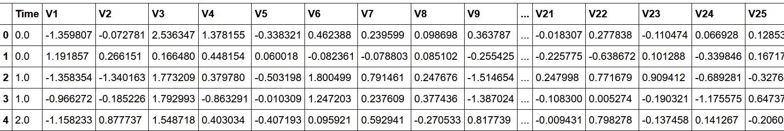
The next step is to read the dataset using the “pd.read_csv()” , followed by the “.head()” command which allows us to view the first five column entries of the dataset along with their respective features.

df_full = pd.read_csv('creditcard.csv')
df_full.head()

Output of the above code:

Visualizing the amount of frauds in comparison to the amount of normal transactions will help us better understand the data.

count_classes = pd.value_counts(df_full['Class'], sort = True)
count_classes.plot(kind = 'bar', rot=0)
plt.title("Transaction class distribution")
plt.xticks(range(2), LABELS)
plt.xlabel("Class")
plt.ylabel("Frequency");

Output of the above code:

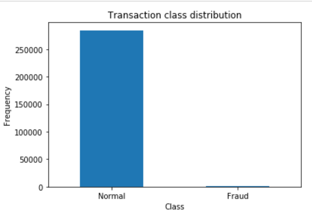
After visualizing the data, we notice that we have a very unbalanced dataset as the normal transactions outweigh the number of frauds committed.

Due to this rarity we perform a stratified sampling on the dataset in order to avoid the result that the model gave as “0” most of the time.

df_full.sort_values(by='Class', ascending=False, inplace=True)
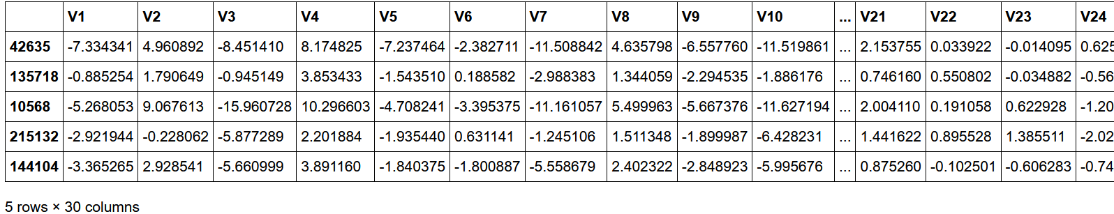
df_full.drop('Time', axis=1,  inplace = True)
df_full.head()

Output of the above code:

Stratified Sampling:

Stratified sampling is a type of sampling method which is used in a large population of data to divide it into small groups or form a subset of the data called as strata in order to organize and finish the sampling process. After the subsets are formed we randomly select the sample proportionally.

This type of sampling is mostly used when we are trying to draw several conclusions from different subsets of data.

df_sample = df_full.iloc[:3000,:]
df_sample.Class.value_counts()

Output of the above code:

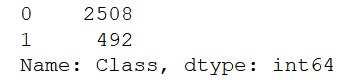
The above code can be used for stratified sampling, it also helps in balancing the ratio between 0 and 1 datasets.

Shuffle the dataset:

The next step to build the dataset is to shuffle the dataset. We shuffle the dataset because by shuffling we can reduce the variance and the bias present in the dataset. Shuffling also is used in order to make sure that the training , testing and the validation sets are representatives of the entire distribution of the dataset.

It also helps with:

1. The process of training which converges fast.
2. It prevents any bias during the training process.
3. It prevents the model from learning the order of the training.

from sklearn.utils import shuffle

shuffle_df = shuffle(df_sample, random_state=42)

df_train = shuffle_df[0:2400]
df_test = shuffle_df[2400:]

train_feature = np.array(df_train.values[:,0:29])
train_label = np.array(df_train.values[:,-1])
test_feature = np.array(df_test.values[:,0:29])
test_label = np.array(df_test.values[:,-1])

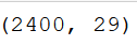
train_feature.shape

Output of the above code is:

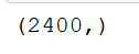
train_label.shape

Output of the above code is:

The code above helps us to shuffle the dataset. We use the “shuffle” keyword present in the sklearn.utils library.

Normalizing the Model:

Normalizing the model means to rescale the values present in the model between the range of [0,1]. In other words , the goal of normalization is to alter the values of the dataset which are numerical in nature without affecting the ranges present in the value or removing or losing information.

It is also known as Min-Max Scaling :

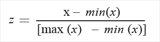
Here the min(x) and max(x) are the minimum and maximum values respectively. Here the minimum value of X is “0” and the maximum value of X is “1”. If the value of X is between minimum and maximum, then the value is between 0 and 1.

from sklearn.preprocessing import MinMaxScaler

scaler = MinMaxScaler()

scaler.fit(train_feature)
train_feature_trans = scaler.transform(train_feature)
test_feature_trans = scaler.transform(test_feature)

The above code will help normalize the values present in the dataset within the range of [0,1].

The neural network:

from keras.models import Sequential
from keras.layers import Dense
from keras.layers import Dropout
import tensorflow as tf

import matplotlib.pyplot as plt 
def show_train_history(train_history,train,validation):
    plt.plot(train_history.history[train])
    plt.plot(train_history.history[validation])
    plt.title('Train History')
    plt.ylabel(train)
    plt.xlabel('Epoch')
    plt.legend(['train', 'validation'], loc='best')
    plt.show()

model = Sequential()
model.add(Dense(units=200, 
                input_dim=29, 
                kernel_initializer='uniform', 
                activation='relu'))
model.add(Dropout(0.5))
model.add(Dense(units=200,  
                kernel_initializer='uniform', 
                activation='relu'))
model.add(Dropout(0.5))
model.add(Dense(units=1,
                kernel_initializer='uniform',
                activation='sigmoid'))

The above code shows the neural network implemented along with the number of layers which are required for the dataset.Here we use the keras framework to build the sequential model. This is a simple 6 layered neural network which gives an accuracy of more than 98%.

print(model.summary())

The output of the following code is:

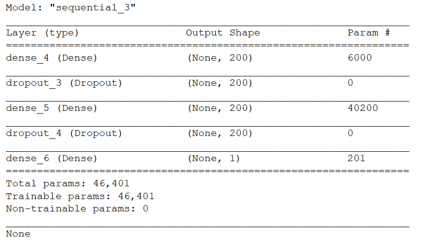
The model.summary() function shows us the summary of the entire model along with the number of parameters present in each layer of the model.

The next step would be to compile the model using the “model.compile” function in which we specify certain parameters such as the “loss” , “optimizer” and “metrics” parameters. Here we use the:

1. Loss Function : “binary_crossentropy” because here we are trying to classify the numerical attributes of the dataset as they are between 0 and 1.
2. Optimizer : “adam” because it helps in bias correction and mostly out-performs the RMSprop towards the end of the optimization process as the gradients become lesser.
3. Metrics : “accuracy” because we need to validate the model.

model.compile(loss='binary_crossentropy',
              optimizer='adam', metrics=['accuracy'])

To progress further, we need to use the “model.fit” method which is :

train_history = model.fit(x=train_feature_trans, y=train_label,
                          validation_split=0.8, epochs=200, 
                          batch_size=500, verbose=2)

The output of the following code is:

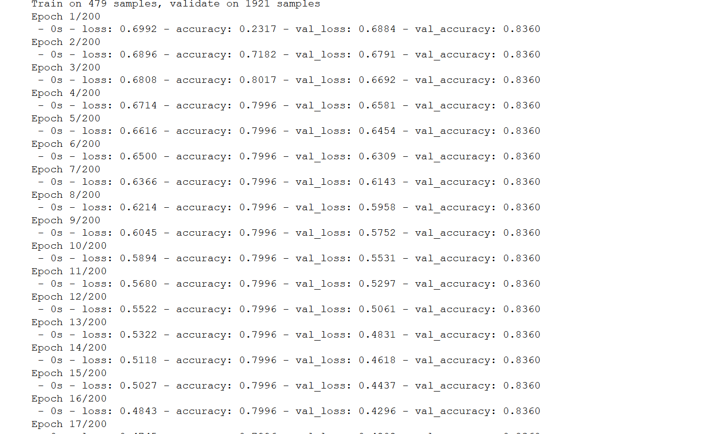
Here in the above code we use the model.fit method specify:

1. The input data to be “x”.
2. The target data to be “y”.
3. We use the “validation_split” to be a value between 0 and 1, otherwise this sets a fraction of the data on which it will evaluate the loss and any model metrics on this data as well.
4. We use the “epochs” to specify the number of iterations over the entire data(x and y) provided.
5. “Batch_size” specifies the numbers of samples to be used every time the gradient updates. If the value is not mentioned then it is taken to be 32 by default.
6. The “verbose” here is set to “2” indicating that we progress only one line per epoch, and 2 is mostly used only when we are running the model non-interactively.

After this step, we move on to plot the accuracy against the validation accuracy in order to make sure that we are progressing in the right way and are not overfitting the data. We also plot the graph between the “loss” and the “validation loss” to track it’s progress.

We use the “model.evaluate” to evaluate the model and figure out if we have used the best parameters for the given problem.It has 3 main arguments which are the test data, test data label and the verbose.

show_train_history(train_history,'accuracy','val_accuracy')
show_train_history(train_history,'loss','val_loss')

scores = model.evaluate(test_feature_trans, test_label)
print('\n')
print('accuracy=',scores[1])

prediction = model.predict_classes(test_feature_trans)

After executing the above code, we observe the following graphs and the accuracy presented.

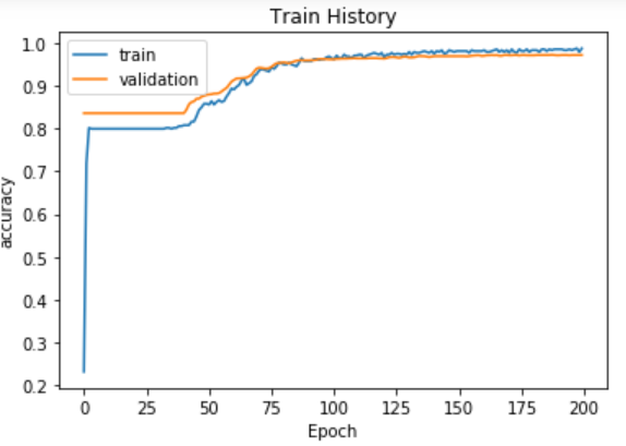
Figure - graph between the accuracy against the validation accuracy

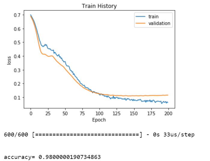
Figure - The graph between “loss” and the “validation loss” along with the accuracy.

Summary:

In this article, we reviewed how neural networks help in detecting frauds in credit card transactions and help in reducing the fraudulent act. These neural networks can also be used in detecting frauds not only in credit card transactions but also in day to day banking activities.

Reference to the Dataset: https://www.kaggle.com/mlg-ulb/creditcardfraud
Github Link: https://github.com/Sandeep-bhuiya/Fraud_detection-Part-1-