In this article at OpenGenus, we will go over the improvements made to traditional Poisson image denoising algorithms using deep learning methods from Po-Yu Liu and Edmund Y. Lam's article of the same name.

The researchers begin by giving a background on what Poisson noise is. They then name the dataset of training images and several traditional poisson denoising algorithms that they plan to use as benchmarks against their deep learning approach. Finally, based on the results of their comparisons, the researchers conclude that the deep learning approach has greater quality based on both statistical metrics and the eye test.

Table of Contents

1. Introduction
2. Poisson Noise Problem
3. Data and Algorithms
   • Training Data
   • Traditional Algorithm
   • Deep Learning Method
4. Results
   • Visual Perception of Output
   • Quantitative Comparison
   • Stride Size and Computational Speed
   • Effects of Noise Strength
5. Conclusion

Introduction

Image reconstruction refers to taking corrupt images and finding the original clean version of the image. Of the various forms of corruption, the focus of the researchers' paper is noise, which visually most gives an image a "granular" looking texture. Although traditionally most algorithms have focused on denoising Gaussian noise, with the increasing prevalence of mobile phones, which come with lower grade sensors, the need to denoise dirty nighttime pictures (Poisson noise) has increased as well. Thus, we arrive at the purpose of this paper: expanding upon existing Poisson denoising methods by trying to apply deep learning to the problem.

Poisson Noise Problem

To start off, the researchers begin by explaining Poisson noise and how it differs from Gaussian Noise. Conceptually Poisson noise is a type of noise that exists mainly at low-light levels and is named as such because it follows a Poisson distribution, which is a discrete probability distribution.

In low light levels there will be a low number of photons hitting a photo sensor, which will determine the brightness of the pixels in the image. As a result, there may be wild variation in the number of photons that hit the sensor at a given moment than in a bright environment, and this level of variation is something that cannot be modeled by a Gaussian (normal) distribution.

Thus, following Poisson distribution equation gives the probability of having x occurrences (photons) hitting the sensor assuming that the occurences happen at an average rate of lambda and that they happen independently of each other.

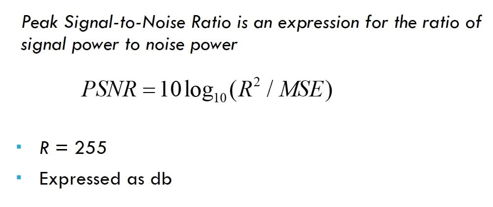
Conventionally, the lambda of the function is considered its peak, and the lower the peak, the stronger the noise of the image. This is corroborated by the signal-to-noise ratio, which is the lambda divided by the standard deviation (square root of lambda), with higher brightness implying a higher ratio (so less noise relatively speaking).

The researchers note that to actually measure the effectiveness of their deep learning model, though, they will be using the peak-signal-to-noise-ratio (PSNR) as a measure of performance instead, which is expressed as the following:

Data and Algorithms

In this section, we will elaborate on the training data set used to train the deep learning model that the researchers proposed, the traditional non-deep learning Poisson denoising method that the model is being benchmarked against, and some of the details of the deep learning model itself.

Training Data

The researchers used the PASCAL Visual Object Classes 2010 images (11321 images) to train their deep learning model. Furthermore, they included another 21 standard test images to be used to evaluate the performance of the model compared to traditional methods. All images were made greyscale to make their use easier in the model. Training set images were divided into 64 64x64 patches of pixels to pass into the deep learning model. Patches larger than 64x64 would go beyond memory/computational constraints.

Traditional Algorithm

For the traditional method, the researchers settled on Block-matching and 3D Filtering (BM3D) with Variance-stabilizing transformation (VST). The BM3D algorithm is a popular Gaussian denoising algorithm that takes a patch of a larger image and looks for similar patches. The patch is then transformed into 3D space and back to 2D space to get the denoised image. As for the VST, it is used to make the Poisson distribution noise approximately Gaussian so as to apply the algorithm. So, distribution is made approximately Gaussian, BM3D is applied, and then the transformation is reversed (inverse transformation) to get the final denoised image.

Deep Learning Method

The deep learning network is comprised of two branches, and each branch itself is comprised of convolutional "compressor" layers and deconvolutional "decompressor" layers. The 64x64 noisy image patches are passed into the input and compared against the corresponding clean version of the patch, which is how the network learns to denoise the image properly. It does so by passing the image patches through a branch, which first compresses the image down to smaller resolutions. By doing so, the statistically nonrepresentative variation in the image (the noise) is removed. Then, the lower resolution patches are then decompressed to reconstruct the original image.

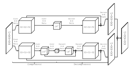
For example, one branch takes the 64 64x64 patches and passes it through two compressor layers, which create 32 32x32 patches and 16 16x16 patches respectively. Then two decompressor layers reverse each of the prior transformations. Inevitably, the repeated compression leads to a loss of image detail, which is why there are two branches. As can be seen in the diagram above, the lower branch has higher compression ratios, which would have a stronger denoising effect at the cost of detail, while the upper branch has lower ratios, which would denoise less in exchange for retaining more image detail.

With both of these branches, the network can have the branches "learn" from each other's strengths, where the stronger denoising branch can learn to retain details from the branch that preserves more detail and vice versa. Furthermore, since the convolution-deconvolutional layers come in pairs, they can also remind the layers further down the pipeline of any lost details and better propagate gradients.

Results

We will now go over what the researchers concluded about the effectiveness of their deep learning Poission denoising model from both a subjective (E.g. eye test) and empirical perspective as well as the model's performance constraints. It should be noted that the images that are being tested have a Poisson noise peak value of 4 and the stride size of the model is 1.

Visual Perception of Output

Based on the several sample images used, the deep learning model is a subtle but noticeable improvement over the non-machine learning BM3D + VST algorithm. The deep learning model produces smoother textures with less erratic color variations than the traditional method. Most importantly, it seems to produce this higher quality without sacrificing much fine detail either as the text in certain images are still clearly distinguishable with the deep learning model as they are with BM3D + VST.

Quantitative Comparison

Numerically (based on PSNR measurements), the deep learning model won out over the non-machine learning benchmark in 18 out of 21 test images used. On average the deep learning model had a 0.38 dB higher PSNR. A two-tail t-test was conducted to verify that this difference was indeed statistically significant and not a byproduct of random chance, implying that it is likely that the deep learning model is indeed more effective.

Stride Size and Computational Speed

The current iteration of the deep learning model takes 20 times longer to operate than the BM3D + VST pair because its stride size is 1. An increase in stride size would increase computational efficiency by reducing the number of patches examined at the cost of quality. In fact, doubling stride size would reduce computational time by 4, and a stride size of between 8 and 32 both runs faster than BM3D + VST while still maintaining improved performance.

Effects of Noise Strength

All of the test images that were used in the experiment had a Poisson peak noise value of 4, however the researchers decided to also examine other noise levels as well. Besides the network trained for value 4, they trained networks for peak values 1, 2, 8, and 16, with the lower peak value implying stronger noise. Once the peak values reach 8 and 16, the deep learning model either barely edges out or performs worse than its non-machine learning counterpart, which demonstrates that the deep learning model performs better in noisier environments.

The researchers believe that this is caused by two possible reasons. One is because when the noise is weak, the effects of the compression done by the deep learning model become more pronounced. Another is because the VST that can transform the Poisson distribution into approximately Gaussian starts breaking down when the mean value goes below 4.

Conclusion

You have learned how a deep learning model can be trained to do Poisson denoising more effectively than traditional methods without being taught any explicit characteristics of the noise in question. Although the current network remains minimalistic and unrefined, deep learning Poisson denoising remains a strong candidate for future Poisson denoising advancements per the article's closing remarks.