Predicting Air Pollution Levels in New Delhi (Part Three)

This is the final part of a three-part series about how I applied Machine Learning to predict pollution levels in New Delhi. Part One introduces the problem, some solutions, and how prediction can help. Part Two focusses on the data we require, and involves initial analysis. In the final part, we go over the implementation of the machine learning model. This entire project is implemented in Python using Jupyter Notebook, and links to the Github repo can be found at the end.

The Approach

The idea was always to use supervised learning - and to treat this as a regression problem rather than a classification problem. In other words, my aim was to predict the value of PM 2.5 at a given date (month) and hour, using the weather features of that hour (temperature, relative humidity, windspeed). A classification problem would use those features to predict a catgeory - perhaps such as "Hazardous", "Unhealthy" and "Good". I wanted to predict the exact value of PM 2.5 instead. We can later use the commonly accepted US definiton of the Air Quality Index to also tell the risk category.

I compared multiple regression models that I will discuss below, but first we must decide what metric will be taken to compare their performance. My goal for this project is to be able to identify the PM 2.5 concentration with a minimal error. The metric I chose is Root Mean Squared Error (RMSE). This is a measure of the average distance my predictions have from the ground truth. It is a popular metric that is commonly used for such tasks.

Loading the Data

To get to know our data and perform the inital analysis and then implement a machine learning model, it first has to be loaded. Pandas dataframes are the go-to for these kinds of data science applications.

import pandas as pd
import numpy as np
import seaborn as sns
import matplotlib.pyplot as plt
import math

# Import CSV file into a dataframe
df = pd.read_csv('final_dataset.csv')
df.head(10)

# Find the number of columns and rows
df.shape

# List of features
df.dtypes

We have 15107 rows and 26 columns in our dataset. This is after we merged both pollution and weather data (after converting pollution data from hourly intervals to three-hour intervals, as discussed in Part Two). We have not cleaned the dataset yet.

The list of features included:

Date
PM2.5
PM10
NO
NO2
NOx
NH3
CO
SO2
O3
AQI
AQI_Category
Month
Day
Hour
Temp
Rel_Humidity
Wind_Direction
Wind_Speed

Cleaning the Data

Since we won't be using all of these features, I will trim the attributes that are not required. This can be done using the drop command:

df2 = df.drop(labels=['PM10', 'NO', 'NO2', 'NOx', 'NH3', 'CO', 'SO2', 'O3','AQI','AQI_Category','Day','Wind_Direction'], axis=1)

After minimiizing the number of features and keeping the ones we need, we're left with this:
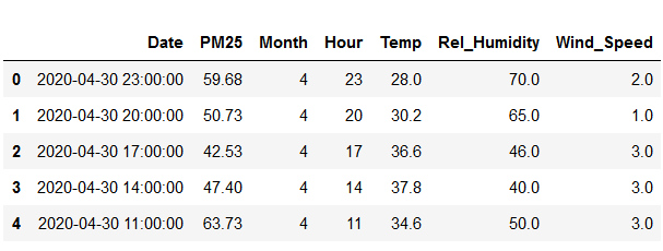
Screenshot_2020-08-27-Air-Quality-Prediction---Delhi---Jupyter-Notebook

The date feature is first converted into a datetime object - Pandas works well with this format and it eliminates ambiguities. This is done using the following code:

import datetime as dt
df['Date'] = pd.to_datetime(df['Date'])

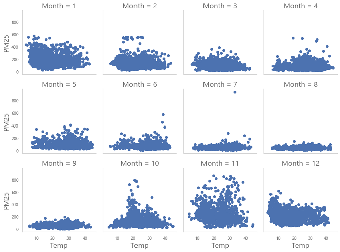
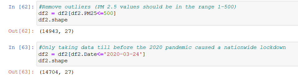
Also, as discussed in Part Two, PM 2.5 levels should not exceed 500. These outlier values need to be removed. Most of the time in really large datasets there will be outliers, erroneous data, or even typos. These can be seen when we make visualizations. For example, in the following visualization of PM 2.5 level variation with temperature for each month:
month-temp

Apart from dropping records with over 500 values for PM 2.5, we shall also not consider the records after 24th March 2020, since the global pandemic lead to a nation-wide lockdown in India at the time. Air quality has seemingly been affected by this, so we do not want our model to take into account this exceptional case.
Screenshot_2020-08-27-Air-Quality-Prediction---Delhi---Jupyter-Notebook-1-

Previous Value Features

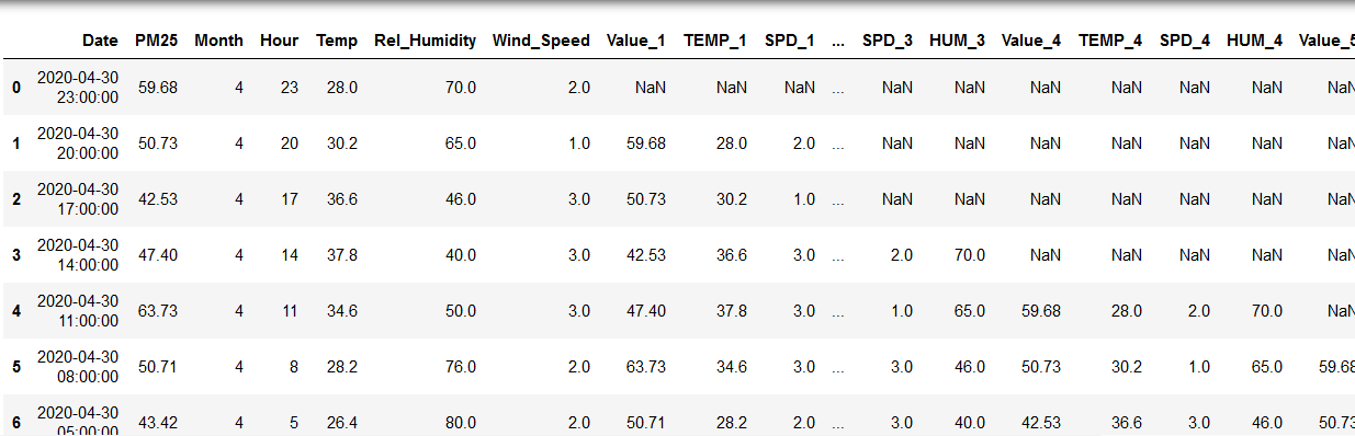
Using weather conditions of the previous 5 instances leading to the current instance will give our model more features to work with and will better improve accuracy. In other words, since the weather conditions at a given time depend on the conditions leading up to that time, we need to include these features in our dataset. We will shift the data and add new columns to list the previous values going back upto 5 hours.

Thus, for temperature, wind speed, humidity and PM 2.5 we shall create columns that give their values 1, 2, 3, 4 and 5 hours before the current hour. For example, Value_1 stands for the PM 2.5 level 1 hour before the current record. Similarly we have the other features.

This is done in Python like this:

# repeat for periods = 2,3,4,5
df2['Value_1'] = df2.PM25.shift(periods=1)
df2['TEMP_1'] = df2.Temp.shift(periods=1)
df2['SPD_1'] = df2.Wind_Speed.shift(periods=1)
df2['HUM_1'] = df2.Rel_Humidity.shift(periods=1)

Things will look like shown below now. Notice the NaN (not a number, empty) values for the first few rows, this is because there are no records for previous instances for these rows. The later rows have complete values however.

shifting

Handling Missing Values

Removing blank values is quite important as many machine learning algorithms can’t use these as inputs. Our dataframe now has a large number of rows with NaN values.

Here is how you can check if your dataset has missing values:

# Are there null values in our dataset?
df2.isnull().values.any()

I dropped some records such as wind speed, which had only a handful of missing values. Dropping records is not ideal, as generally more records means better accuracy for a machine learning model, but it is simple to do. For other features that had plenty of missing values, such as the newly created previous value features, I took another approach.

There are various ways to fill or impute missing values: forward fill, back fill, or just taking the mean. I used forward fill, which is achieved in Python like this:

#Forward filling
df2['Value_1'] = df2.Value_1.fillna(method='ffill')
df2.HUM_1.fillna(method='ffill')
df2['TEMP_1'] = df2.TEMP_1.fillna(method='ffill')

Now again we check to see if the dataset has any NaN values after all of this cleaning. Great, we don't! Let's see how many records we have left using data.shape

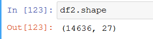
Screenshot_2020-08-27-Air-Quality-Prediction---Delhi---Jupyter-Notebook-1

We still have plenty of records to work with, and the number of columns has increased. Now the list of columns consists of:

Date
PM25
Month
Hour
Temp
Rel_Humidity
Wind_Speed
Value_1
TEMP_1
SPD_1
HUM_1
Value_2
TEMP_2
SPD_2
HUM_2
Value_3
TEMP_3
SPD_3
HUM_3
Value_4
TEMP_4
SPD_4
HUM_4
Value_5
TEMP_5
SPD_5
HUM_5

Now we have a clean dataset with no missing values or outliers.

Splitting into training and testing data

Before we actually implement a few models, we need to split the data. We keep 30% of it aside for later. We shall use 70% of it to train these models, and test them against the portion kept aside. Cross-validation like this is always desired when training machine learning models to be able to trust the generality of the model created.

from sklearn.model_selection import train_test_split

y = data['PM25']
X = data.drop(['PM25'], axis=1)
X_train, X_test, y_train, y_test = train_test_split(X, y, test_size=.3, random_state=1234)

X_train.shape, y_train.shape
X_test.shape, y_test.shape

This yields 10245 training rows and 4391 rows for testing.
Now, our target variable is y (the PM 2.5 level), and X is the remaining featureset. We have split our data using an inbuilt function available in sklearn.

We can now get into the meat of this post and build a couple of regression models!

ML Models

We will try a couple of models and see how well they perform. The easiest to understand is simple Linear Regression, so I did that first. I implemented two models I am most familiar with - simple Linear Regression and then Random Forest Regressor. Let us see which performed better:

Simple Linear Regression Implementation

from sklearn.linear_model import LinearRegression
from sklearn.metrics import mean_squared_error, mean_absolute_error, r2_score

# Create linear regression object
regr = LinearRegression()

# Train the model using the training set
regr.fit(X_train, y_train)
# Make predictions using the testing set
lin_pred = regr.predict(X_test)

from math import sqrt
# The coefficients
print('Coefficients: \n', regr.coef_)
# The mean squared error
print("Root mean squared error: %.2f"
      % sqrt(mean_squared_error(y_test, lin_pred)))

These were the results:
Root mean squared error: 45.27
Mean absolute error: 28.68
R-squared: 0.74

Random Forest Regression Implementation

from sklearn.ensemble import RandomForestRegressor
from sklearn.metrics import mean_squared_error, mean_absolute_error, r2_score


# Create Random Forrest Regressor object
regr_rf = RandomForestRegressor(n_estimators=200, random_state=1234)

# Make predictions using the testing set
regr_rf_pred = regr_rf.predict(X_test)

# The mean squared error
print("Root mean squared error: %.2f"
      % sqrt(mean_squared_error(y_test, regr_rf_pred)))

These were the results:
Root mean squared error: 40.03
Mean absolute error: 24.95
R-squared: 0.80

Random-Forest-Regressor

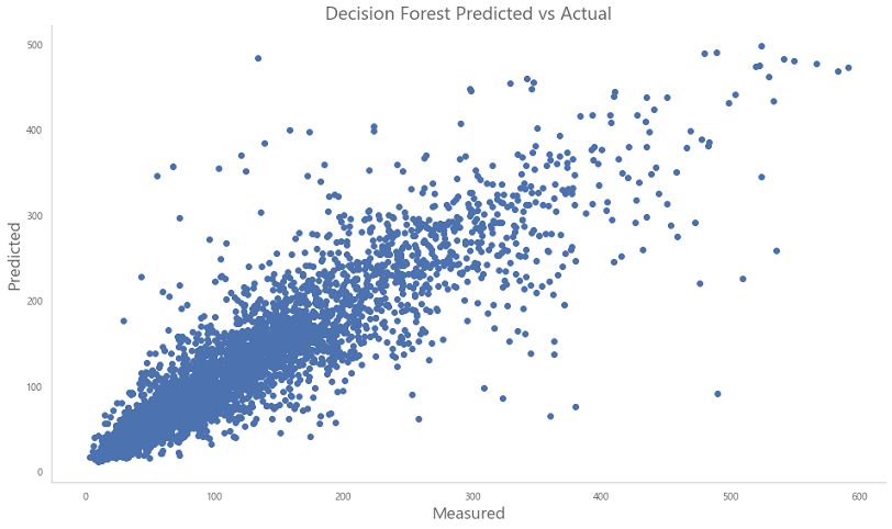
With an RMSE of about 40, and an coefficient of determination at 0.8, the Random Forest Regressor outperforms the Linear Regression model slightly. Using Boosting based techniques, such as Adaboost or XGBoost, we can further reduce our RMSE. That is something for me to try out in the future.

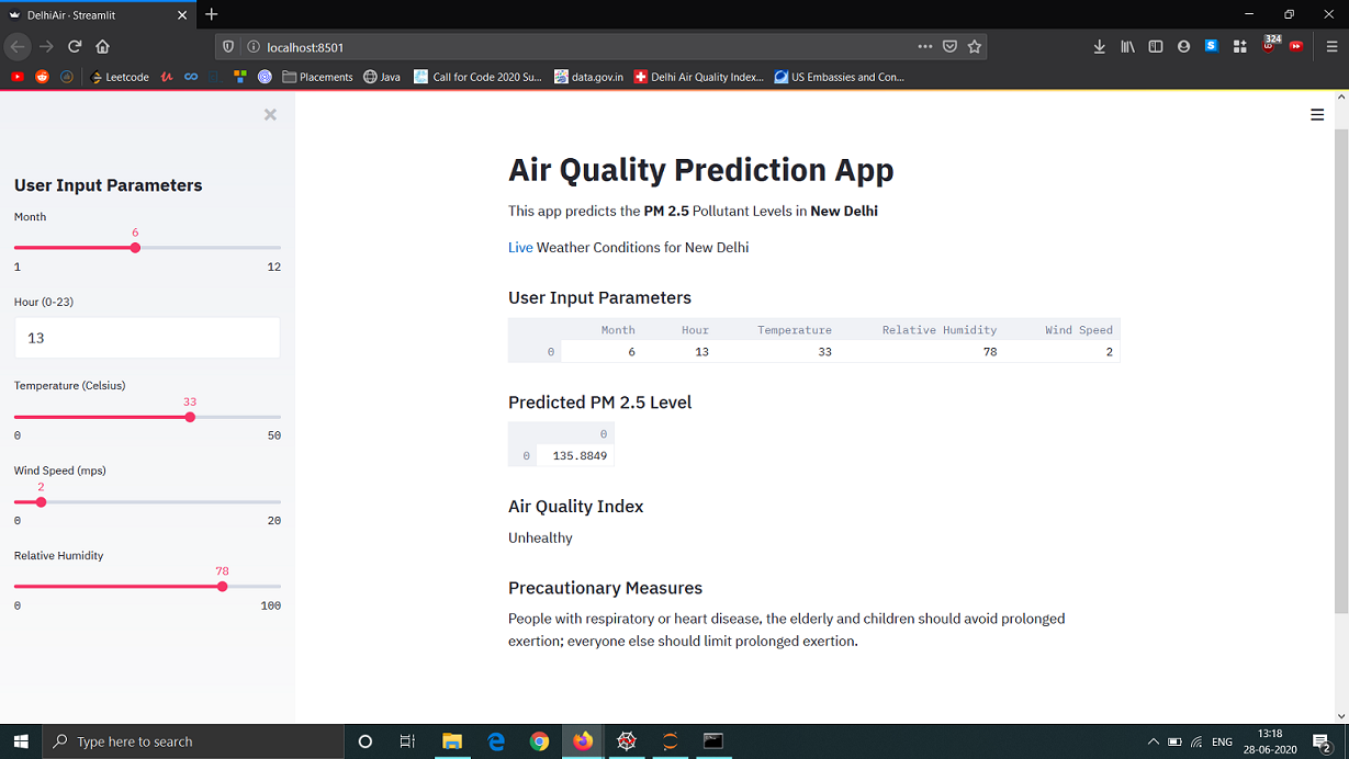
To try something new, I decided to convert this Jupyter Notebook implementation into a web application. While I will not go into the implementation details here, it is fairly simple using Python libraries such as Streamlit. I used it to display the predicted PM 2.5 level and corresponding AQI value, and also mention the risks and preventive measures. The user has to input the time and month, and the current weather conditions. Given that we relied on Safdarjung weather station data, our model should be most accurate for that part of New Delhi.

Here is what it looks like:
web-app

Final Words

Thank you for going through this three-part series where I discussed a problem my city faces, and tried to help solve one aspect of it using a Machine Learning approach. Overall our model showed acceptable results, but going forward one should aim for a RMSE below 30. Going further, to make this a widely-acccesible product that can help people in the capital region, I would have to learn how to deploy it using a service such as Azure.

Please stay safe and help prevent air pollution by carpooling and using public transport like the Delhi Metro and CNG bus network. Walk or bicycle small distances, and wear a mask in winter months!