Softmax function and layers are used for ML problems dealing with multi-class outputs. This idea is an extension of Logistic Regression used for classification problems, which, for an input, returns a real number between 0 and 1.0 for each class; effectively predicting the probability of an output class.

Softmax extends this idea to multiple classes. Softmax, similar to its contemporary Logistic Regression, outputs a series of decimals between 0 and 1.0 for each output class that has been trained upon.

For example, if you are an owner of a warehouse which stores 3 variety of fruits - apple, mango and pineapple. Now, every consignment that you receive contains a mix of these 3 fruits. You have installed a scanning machine which uses a softmax classifier to classify and segregate the different fruits.

So, if it encounters a fruit something similar to this

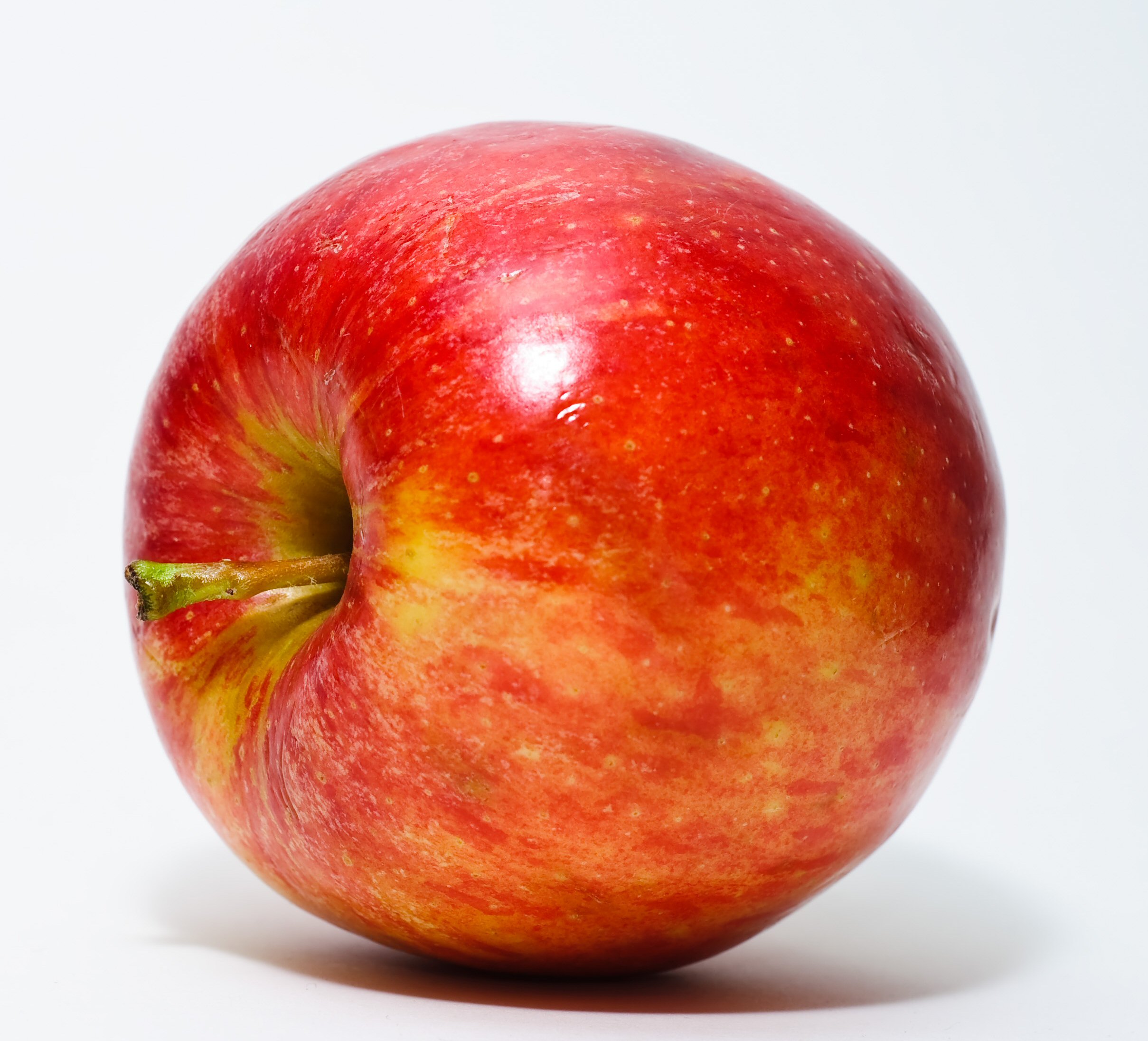
It will generate an output similar to this -

Class	Probability
Apple	0.96
Mango	0.03
Pineapple	0.01

This classifier will return Apple as output and rightly so. One thing to notice here is how the sum of probabilities of all classes is equal to 1.0, similar to Logistic Regression classification.

We will implement it using Tensorflow's Sequential API. We are going to work on Kaggle's flowers dataset. While it is originally a 17 class dataset, for the sake of simplicity we will deal with only 3 different classes (Daffodil, Snowdrop and Lily Valley). Each class contain 80 different images which will later be split into training and validation set. You can find the same here.

Softmax Regression is generally implemented in the following steps -

1. One-Hot Encoding of training targets.
2. Implementing a Neural Network Model with a Softmax layer as the output layer.
3. Compiling the model with an appropriate loss function and an optimizer.
4. Fitting on the training and predicting on the validation set.

Before implementing Softmax Layers, let us first understand what Softmax Function is and how does it compute probabilities of different output classes.

Softmax Function

The mathematical expression of softmax looks something like this -

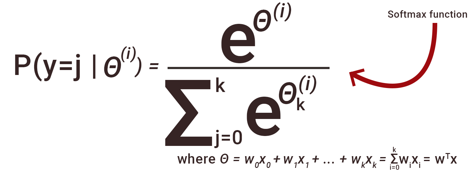
Now, the graphic tells us how output probabilities are computed.

On the one-hot encoded logits(a bunch of numbers computed for each of the respective classes) of a single neuron of the Dense layer, the softmax function is applied. Such is the nature of the function that all the outputs will be between 0 and 1, thus essentially providing us with the probabilities for different classes. The one with the highest probability is taken as the output.
Following is the psuedocode for implementing softmax -

        1.One hot encode your training targets.
        2.Compute the logits or the unnormalised predictions from training data.
        3.Apply Softmax function as given above to the logits.
        4.Compute the loss using cross-entropy.
        5.Apply Optimization. 

This can be implemented in Python using this code -

         def softmax(x):
             """Compute softmax values for each sets of scores in x."""
             e = []
             for t in x:
               e_x = np.exp(t - np.max(t))
               e.append(e_x / e_x.sum())
             e = np.array(e)   
             return e
          
          #test
          l = [1.0,2.4,5.6]
          softmax(l)

Result

          array([0.00956576, 0.03879107, 0.95164317])

One-Hot encoded matrix form is a representation that shows the probabilities of all classes pertaining to the observation. Taking our previous example, for a training image of a Pineapple it will have a training class 2. This can be represented in the following way - [0,0,1]. This highlights that the probability of the image being in any one of the 3 classes. Clearly, the probabilities of Apple and Mango class are 0 while that of pineapple is 1.

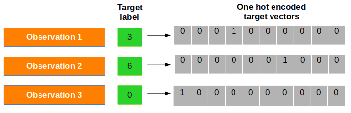
One-hot encoded form can be implented using tf.keras.utils.to_categorical(y, num_classes= number_of_classes)

Cost Function

Now, in order to gauge our model prediction with the actual target variables, we need a cost function. It's generally the Cross Entropy. Cross-entropy or Log Loss is a distance calculation function which takes the probabilities from the softmax layer and the created one-hot-encoding target matrix to calculate the distance. Since in classification problems, we need to determine the class of an unseen item, we need to find the prediction class with the smallest distance between the actual class and itself. And thus we need to minimize this loss for accurately predicting on unseen data.

To get started we define D(S(i)|T(i)), where S(i) is a vector of calculated probabilities for the ith observation and T(i) is the one-hot encoded vector of the target output class of the ith observation.

The cost function is then formulated -

The code for implementing the cross-entropy cost function is the following -

    total_loss = -tf.reduce_sum(y_true * tf.math.log(),axis = [1])

The same can be implemented using Tensorflow library as well -

    tf.nn.softmax_cross_entropy_with_logits(labels=y_true,logits=y_pred)

It is therefore clear that for the right target classes, the distance values will be lesser, and the distance values will be more significant for the wrong target classes. Now, the task in hand is to minimize this cost using a suitable optimizer. Optimization algorithms like Stochastic Gradient Decent compute gradients of the cost function with respect to the weights and then subtract them with the respective weights. tf.optimizers.SGD(0.05) is generally used to implement Stochastic Gradient Decent.

All this is done at the end of each forward cycle and the gradients are passed on for updating or learning of the weights in the backward cycle. This way, we aim to minimize the cost and push up our prediction accuracy.

Step-by-Step Implementation

So, if someone wishes to step-by-step implement softmax classification, they can do it using Tensorflow's Gradient Tape approach. Make sure to convert your training labels to one-hot encoded form before proceeding -

    # Model Class
    class Model(object):
        def __init__(self, x, y):
           # Initializing the weights and the biases
           self.W = tf.Variable(tf.random.truncated_normal([num_features, num_labels])) 
           self.b = tf.Variable(tf.zeros([num_labels])) 

        def __call__(self, x):
           return tf.matmul(x, self.W) + self.b


    #Loss Function
    def loss(predicted_y, desired_y):
            
            return tf.reduce_mean(tf.nn.softmax_cross_entropy_with_logits(labels=desired_y,logits=predicted_y))
         
         
 #SGD Optimizer
 optimizer = tf.optimizers.SGD(learning_rate)


 #Training gradients using Gradient Tape and applying it to the optimizer
 def train(model, inputs, outputs):
     with tf.GradientTape() as t:
        current_loss = loss(model(inputs), outputs)
     grads = t.gradient(current_loss, [model.W, model.b])
     optimizer.apply_gradients(zip(grads,[model.W, model.b]))
     print(current_loss)    


 #Creating instances of model class 
 model = Model(x_train, y_train)


 #Training 
 for i in range(num_epochs):
     train(model,x_train,y_labels)

Sequential API Implementation

Implementation of a Softmax layer in a Neural Network Model is a relatively simple task, thanks to the Sequential API of Keras and its Dense Layers. Our very first task is to import the required libraries. Since we are performing an Image Classification, we will use the Convolutional Layer and Pooling layer. However, since we are doing a multi-class classification, we will use a Keras Dense Layer with "softmax" activation function as the output layer. All of them can be imported from tensorflow.keras.layers.

    import keras
    from keras.models import Sequential
    from keras.layers import Dense, Dropout, Flatten
    from keras.layers import Conv2D, MaxPooling2D
    from keras.utils import to_categorical
    from keras.preprocessing import image
    import numpy as np
    import pandas as pd
    import matplotlib.pyplot as plt
    from sklearn.model_selection import train_test_split
    from keras.utils import to_categoric
    al

Now we have to import our data into our workbook. If you are using a Jupyter Notebook, you can move your data in the specific directory. If you are using a Colab Notebook, then you can manually import your data.

    from google.colab import files
    files.upload()

After importing the required files, you have to assign them to convert them in a machine-understandable form and assign it to X and y.

      # "files.txt" contains the order-wise name of all the image files. 
      train = pd.read_fwf('files.txt',header = None)
      train = train.loc[0:240,0]
      
      #We will use the training images in a 64*64*3 format.
      train_image = []
      for i in range(240):
        img = image.load_img(train[i], target_size=(64,64,3))
        img = image.img_to_array(img)
        img = img/255
        train_image.append(img)
      X = np.array(train_image)
      
     #Creation of target set.Each of the 3 classes have 80 photographs arranged          in a sequencial manner.
     y = []
      for x in range(240):
        if(x<80):
          y.append(0)
        if(80<= x <160):
          y.append(1)
        if(160<= x<240):
          y.append(2)

Now it is essential to convert our target variables into one-hot encoded vector form. We will use the to_categorical function of Keras library for this.

      y_final = to_categorical(y)
      y_final

Result

     array([[1., 0., 0.],[1., 0., 0.],[1., 0., 0.],[1., 0., 0.],.....[0., 0., 1.],[0., 0., 1.],[0., 0., 1.]], dtype=float32)

Now with our data ready, its time to implement our classification model. Therefore, we will split the training and test sets, build and compile our Sequential model with appropriate layers, loss functions and optimizers and then fit our model on our training set. We will use the test set for validation.

      #Splitting our training and test sets
      X_train, X_test, y_train, y_test = train_test_split(X, y_fall, random_state=42, test_size=0.2)
      
      #Building our Sequential model
      model = Sequential()
      model.add(Conv2D(32, kernel_size=(3, 3),activation='relu',input_shape=(64,64,3)))
      model.add(Conv2D(64, (3, 3), activation='relu'))
      model.add(MaxPooling2D(pool_size=(2, 2)))
      model.add(Dropout(0.25))
      model.add(Flatten())
      model.add(Dense(128, activation='relu'))
      model.add(Dropout(0.5))
      model.add(Dense(3, activation='softmax'))
      
      #Compiling our model with appropriate loss function and optimizer
      model.compile(loss = 'categorical_crossentropy', optimizer= 'adam',metrics=['accuracy'])
      
      #Fitting the model
      model.fit(X_train, y_train, epochs=10, validation_data=(X_test, y_test))

Note that the type and number of layers as well as number of neurons and activation functions in the layers(except the output layer) is an arbitrary choice. You can choose them according to your use cases. Here we chose the convolutional layers as we are dealing with image data. The important thing to note here is the number of neurons in the output layer is the same as the number of classes in the target variable. This is because our model will predict the probabilities of the happening of those classes. We will specify the activation parameter as "softmax".

As we have discussed earlier, cross-entropy will be the loss/cost function for our model. We will use "categorical_crossentropy" as there are more than 2 classes.

After fitting, we will see something like this.

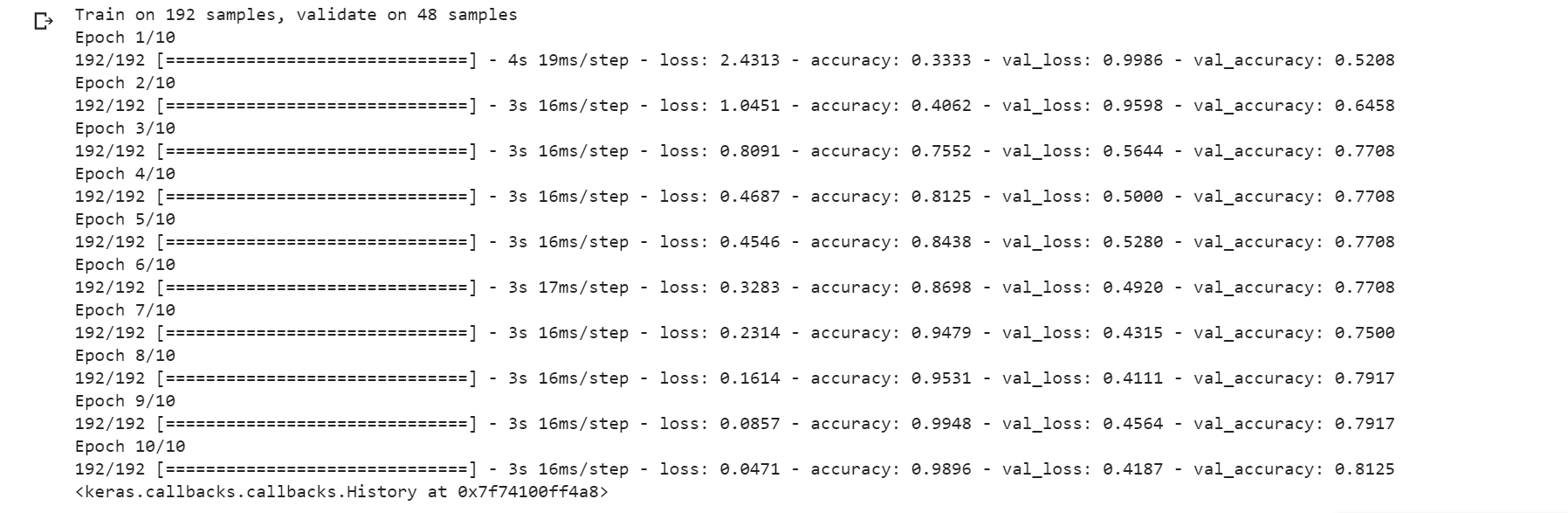
Well, a 98% training accuracy and an 81% testing accuracy is by no means bad! However, it is easy to see that our model overfits (High training accuracy and more reduced test accuracy) and while there are methods to fix it, they are out of the scope of this article.

Now, let's try out our model with a random picture. We will use this picture of the delightful Snowdrop flower.

Let's load it and convert it into an array of numbers and predict our model's output.

       test_img = image.load_img('snowdrop.jpg', target_size=(64,64,3))
       test_img = image.img_to_array(test_img)
       test_img = test_img/255
       
       test_img = np.array([test_img])
      
       y_pred = model.predict_classes(test_img)
       prob = model.predict(test_img)
       
       print("Our predicted class is " + str(y_pred))
       print("The probabilities for our image are " + str(prob))

Result

       Our predicted class is [1]
       The probabilities for our image are [[0.01806867 0.8457334  0.13619795]]

Eureka! Our model correctly predicts which kind our flower is. You can see that the probability for the second class is the highest and hence the model assigns it as the answer.

Similar to our flower classification task, Softmax Layers find their usage in many spheres of Image Processing and Natural Language Processing.

There is an important thing to note; it is crucial to understand where to use Softmax. Softmax is applied for multi-class problems when the different classes are mutually exclusive. For example, you are implementing code for an image classification problem where you have to classify an image into 3 different categories - cat, a black and white image and a man standing. In this situation, the classes are not mutually exclusive as an image can be both black and white as well as have a man or cat in it. Here, K Binary Classification or using K different binary/logistic classifiers (K=3 in this case) will yield better performance as the program can better differentiate among the images.

This introduction to Softmax should be ideal for you to understand and implement it in your capacity.