MFCC (Mel Frequency Cepstral Coefficients) for Audio format

Mel Frequency Cepstral Co-efficients (MFCC) is an internal audio representation format which is easy to work on. This is similar to JPG format for images. We have demonstrated the ideas of MFCC with code examples.
For better understanding of this article you are requested to read these 2 articles:
For study of audio for different results one need to understand various features of audio and then make prediction or understand about your audio.
This task was simplified by Davis and Mermelstein in the 1980's when they introduced the world with Mel Frequency Cepstral Coefficents (MFCCs) as a feature which is now widely used for audio analysis.
First things first what does MFCC stands for it is an acronym for Mel Frequency Cepstral Co-efficients which are the coefficients that collectively make up an MFC. MFC is a representation of the short-term power spectrum of a sound, based on a linear cosine transform of a log power spectrum on a nonlinear mel scale of frequency.
To understand the above statments we define some terms below:
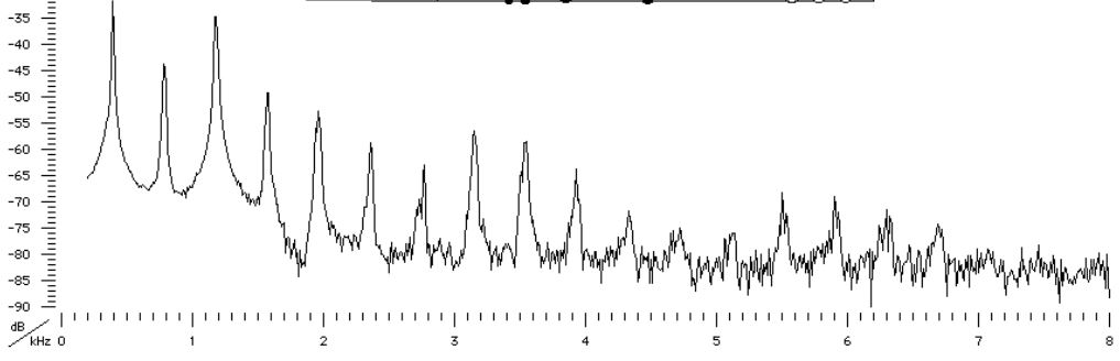
Sound Spectrum : A sound spectrum is a representation of a sound – usually a short sample of a sound – in terms of the amount of vibration at each individual frequency. It is usually presented as a graph of power as a function of frequency.
Linear cosine transform : They can also be called as sine and cosine tranforms which can be easily calculated using fourier transform. During our converion we will be needing both short time and fast time fourier tranform ar different stages.
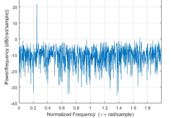
Power Spectrum : It is the result of fourier tranform which we get as a representation.Also known as periodogram.
Mel Scale : Mel scale is a scale that relates the perceived frequency of a tone to the actual measured frequency. It scales the frequency in order to match more closely what the human ear can hear .
A frequency measured in Hertz (f) can be converted to the Mel scale using the following formula :
==Mel(f) = 2595log(1 + f/700)==
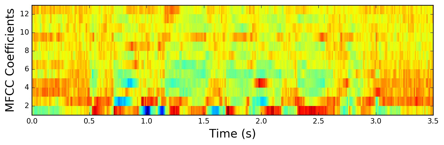
This is how your MFCC may look like
But how to get this? Stay tuned you will not only get the required libROSE feature for this but also a step wise explanation of what actually takes place.
NOTE : Humans are better at identifying small changes in speech at lower frequencies).
Steps to convert audio in MFCC :
NOTE : All the new terms in a step are either explained in the articles mentioned or just below the step!
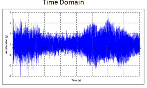
1) Get your audio in a time domain format.
2) Covert your audio in a periodogram with the help of Fast Fourier Tranform. We do so as it will give us a Nyquist frequency by downsampling of your audio so that we can identufy the sound.
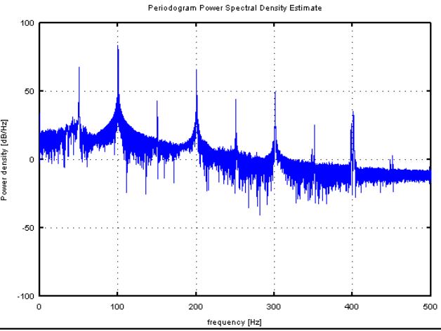
A periodogram is similar to the Fourier Transform, but is optimized for unevenly time-sampled data, and for different shapes in periodic signals. (Pictoral representation is shown later in this article)
In order to recover all Fourier components of a periodic waveform, it is necessary to use a sampling rate nu at least twice the highest waveform frequency. The Nyquist frequency, also called the Nyquist limit, is the highest frequency that can be coded at a given sampling rate in order to be able to fully reconstruct the signal, i.e.,
f_(Nyquist)=1/2nu.
A fast Fourier transform (FFT) is an algorithm that computes the discrete Fourier transform (DFT) of a sequence, or its inverse (IDFT). Fourier analysis converts a signal from its original domain (often time or space) to a representation in the frequency domain and vice versa.
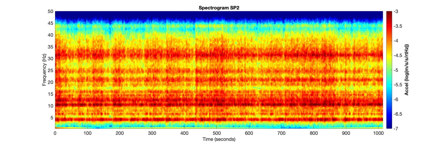
3) After this we convert our periodogram into spectrogram(they are periodograms at different intervals stacked together).
4) Then we perform Short Fourier Tranform idea behind performing this is that it helps us to study a short interval of audio which is assumed to be steady.
The short-time Fourier transform (STFT), is a Fourier-related transform used to determine the sinusoidal frequency and phase content of local sections of a signal as it changes over time.
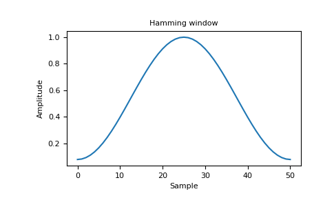
5) Then we perform hamming window (The Hamming window is an extension of the Hann window in the sense that it is a raised cosine window of the form) to prevent spectral leakage(Spectral Leakage is a a phenomenon that takes place due finite windowing of the data. Generally when we take data and pass it to the DFT/FFT algorithm ).
6) We then again perform Fast Fourier Transform to convert amplitude into frequency.
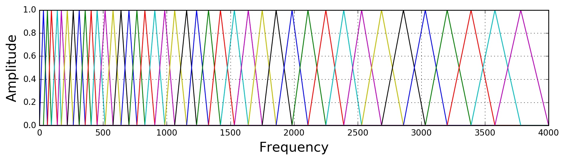
7) Now we convert our frequency into mel scale as they are of better use as discussed above this is done by providing a 26 filter which is defined by macine itself and this help in you machine to learn.
8) Then we perform logarithm of all filterbank energies.
Filter bank is an array of band-pass filters that separates the input signal into multiple components, each one carrying a single frequency sub-band of the original signal
9) Perform IDCT of the log filterbank energies.
10) Keep IDCT coefficients 2-13, discard the rest of the coffecients(12-13 are considered to be the best).
librosa.core.load(path, sr=22050, mono=True, offset=0.0, duration=None, dtype=<class 'numpy.float32'>, res_type='kaiser_best')
NOTE : Since librosa.feature.mfcc accepts a parameter in numpy form one need to convert the audio file with .wav or any other extension to an array which is done by using 2 of libROSA features
Load an audio file as a floating point time series.Audio will be automatically resampled to the given rate (default sr=22050).To preserve the native sampling rate of the file, use sr=None.
Parameters:
path:string, int, or file-like object
path to the input file.
Any codec supported by soundfile or audioread will work.
If the codec is supported by soundfile, then path can also be an open file descriptor (int), or any object implementing Python’s file interface.
If the codec is not supported by soundfile (e.g., MP3), then only string file paths are supported.
sr:number > 0 [scalar]
target sampling rate
‘None’ uses the native sampling rate
mono:bool
convert signal to mono
offset:float
start reading after this time (in seconds)
duration:float
only load up to this much audio (in seconds)
dtype:numeric type
data type of y
res_type:str
resample type (see note)
Example :
>>Load an ogg vorbis file
>>filename = librosa.util.example_audio_file()
>>y, sr = librosa.load(filename)
>>y
>>array([ -4.756e-06,  -6.020e-06, ...,  -1.040e-06,   0.000e+00], dtype=float32)
>>sr
>>22050
NOTE : You don't need to specify all the parameters
**librosa.core.resample(y, orig_sr, target_sr, res_type='kaiser_best', fix=True, scale=False, kwargs)
Resample a time series from orig_sr to target_sr
Parameters:
y:np.ndarray [shape=(n,) or shape=(2, n)]
audio time series. Can be mono or stereo.
orig_sr:number > 0 [scalar]
original sampling rate of y
target_sr:number > 0 [scalar]
target sampling rate
res_type:str
resample type (see note)
Note :By default, this uses resampy’s high-quality mode (‘kaiser_best’).
To use a faster method, set res_type=’kaiser_fast’.
To use scipy.signal.resample, set res_type=’fft’ or res_type=’scipy’.
To use scipy.signal.resample_poly, set res_type=’polyphase’.
Note :When using res_type=’polyphase’, only integer sampling rates are supported.
fix:bool
adjust the length of the resampled signal to be of size exactly ceil(target_sr * len(y) / orig_sr)
scale:bool
Scale the resampled signal so that y and y_hat have approximately equal total energy.
kwargs:additional keyword arguments
If fix==True, additional keyword arguments to pass to librosa.util.fix_length.
Returns:
y_hat:np.ndarray [shape=(n * target_sr / orig_sr,)]
y resampled from orig_sr to target_sr
Example
>>y, sr = librosa.load(librosa.util.example_audio_file(), sr=22050)
>>y_8k = librosa.resample(y, sr, 8000)
>>y.shape, y_8k.shape
>>((1355168,), (491671,))
NOTE : You don't need to specify all the parameters
librosa.feature.mfcc(y=None, sr=22050, S=None, n_mfcc=20, dct_type=2, norm='ortho', kwargs)
Parameters :
y:np.ndarray [shape=(n,)] or None
audio time series
sr:number > 0 [scalar]
sampling rate of y
S:np.ndarray [shape=(d, t)] or None
log-power Mel spectrogram
n_mfcc: int > 0 [scalar]
number of MFCCs to return
dct_type:None, or {1, 2, 3}
Discrete cosine transform (DCT) type. By default, DCT type-2 is used.
norm:None or ‘ortho’
If dct_type is 2 or 3, setting norm=’ortho’ uses an ortho-normal DCT basis.
Normalization is not supported for dct_type=1.
kwargs:additional keyword arguments
Arguments to melspectrogram, if operating on time series input
Returns:
M:np.ndarray [shape=(n_mfcc, t)]
MFCC sequence
NOTE : You don't need to specify all the parameters
In order to perform libROSA features you need numpy as well which can be easily intalled using pip install numpy
Example
import librosa
import numpy as np
import numpy as geek

RATE = 24000
N_MFCC = 13

def get_wav(language_num):
    '''
    Load wav file from disk and down-samples to RATE
    :param language_num (list): list of file names
    :return (numpy array): Down-sampled wav file
    '''

    y, sr = librosa.load('./{}.wav'.format(language_num)) #Make sure to have audio file in your desktop or you may change the path as per your need
    return(librosa.core.resample(y=y,orig_sr=sr,target_sr=RATE, scale=True))

def to_mfcc(wav):
    '''
    Converts wav file to Mel Frequency Ceptral Coefficients
    :param wav (numpy array): Wav form
    :return (2d numpy array: MFCC
    '''
    return(librosa.feature.mfcc(y=wav, sr=RATE, n_mfcc=N_MFCC))

if __name__ == '__main__':

    audio = 'arabic6'
    X= get_wav(audio)
    print(X.shape)#(754141,)
    X=to_mfcc(X)
    print(X.shape)#(13, 1473)

    c = geek.savetxt('file.txt', X, delimiter =', ')
    a = open("file.txt", 'r')# open file in read mode

    #print("the file contains:")
    #print(a.read())
NOTE : The output of this code will be a file.txt which will be created in your system only. Since the contents of this file are large we have attached the file in github repository linked below with same file name as mentioned.