
Get this book -> Problems on Array: For Interviews and Competitive Programming
Scheduling and selection of registers during execution assumes infinite number of registers even though processors only have a limited number of registers, in this article we take a look how variables are mapped onto registers.
Table of contents.
- Introduction.
- Liveness.
- Liveness analysis.
- Interference.
- Register Allocation by graph coloring.
- Spilling
- Heuristics.
- Summary.
- References.
Introduction.
During machine code generation phase in compiler design we translate variables in the intermediate language one-to-one into registers in the machine language.
A concern is that processors don't have an unlimited number of registers therefore we introduce the concept of register allocation for handing these situations.
More formally, register allocation is the mapping of a large number of variables into a limited number of registers.
This is done by sharing the limited number of registers among several variables and when the variables are too many some variables will be stored in memory temporarily, this is called spilling.
Register allocation can be done in either the intermediate code generation phase or the machine code generation phase.
Register allocation during intermediate code generation has the advantage that the register allocator can be used for several target machines by parameterizing with the available set of registers.
However when intermediate code needs translation, we need extra registers for storage of temporary variables.
Machine code uses symbolic names for registers which are converted to register numbers during register allocation. Register allocation after machine code generation has an advantage which can be seen whereby several instructions are combined into a single instruction hence variables disappear and therefore there is no need for allocation.
Techniques for register allocation into machine code generation or intermediate code generation phase are similar.
Liveness.
A variable is live in the program if the value contained might be potentially used in future computations. Conversely it is dead if there are no ways that it can be used for future computations.
Two variables can only share a register if they are both dead, that is, there is no point in the program where they are both live.
Determining if a variable is live.
- It is live if an instruction uses the contents of that variable.(generating liveness)
- If a variable is assigned a value in an instruction while it is not used as an operand in that instruction then its is dead at the start of the instruction.(killing liveness)
- A variable is live at the end of the instruction if it is live at the start of any of the immediate succeeding instructions.(propagating liveness).
- If a variable is live at the end of an instruction and the instruction doesn't assign a value to the variable, then the variable is considered live at the start of the instruction.(propagating liveness).
Liveness Analysis.
This is the process of determining if a variable is live and to do this we formalize rules as equations over sets of variables and solve the equations.
Instructions will have successors - instructions that follow the current instruction during execution.
We denote set of successors for i as succ[i].
Rules for finding succ[i]
- The instruction j listed after instruction i is in succ[i], unless i is a GOTO of IF-THEN-ELSE instruction.
- If instruction i is in the form of GOTO l, the instruction LABEL l is in succ[i]. In a correct program there exists exactly one LABEL instruction with the label used by the GOTO instruction.
- If instruction i is IF p THEN ELSE are in succ[i].
For correct analysis we assume that the outcomes of an IF-THEN-ELSE instruction are possible.
If the above is not upheld this may result in the analysis claiming a variable is live when in fact it is dead which is worse because we may overwrite a value that could be used later and therefore a program may produce incorrect results.
Correct liveness information is dependent on knowing paths a program takes when executed which is not possible to compute with precision therefore we shall allow imprecise results as long as we err on the side of safety(calling a variable live unless we have proof it is dead).
We have set gen[i] which is a set of variables that an instruction i generates liveness for.
We have kill[i] which is a list of variables that may be assigned values by the instructions.
Examples of gen and kill sets for instructions in intermediate code.
| Instruction i | gen[i] | kill[i] |
|---|---|---|
| LABEL l | ∅ | ∅ |
| x := y | {y} | {x} |
| x := k | ∅ | {x} |
| x := unpop y | {y} | {x} |
| x := unop k | ∅ | {x} |
| x := y binpop z | {y, z} | {x} |
| x := y binpop k | {y} | {x} |
| x := M[y] | {y} | {x} |
| x := M[k] | ∅ | {x} |
| M[x] := y | {x, y} | ∅ |
| M[k] := y | {y} | ∅ |
| GOTO l | ∅ | ∅ |
| IF x relop y THEN ELSE | {x, y} | ∅ |
| x := CALL f(args) | args | {x} |
x, y, and z are possibly identical variables.
k denotes a constant.
For each instruction i, two sets will hold the liveness information.
If in[i] holds variables that are live at the start of i and out[i] holds variables that are live at the end of i, we define them using the following recursive equations.
int[i] = gen[i] ∪ (out[i] \ kill[i])
out[i] = in[j].
Since the above equations are recursive we solve them using fixed-point iteration.
First we initialize all in[i] and out[i] to empty sets ∅ and repeatedly calculate new values for these until no further changes occur.
Changes will stop occurring because the sets have a finite number of possible values and adding elements to sets in[i] or out[i] on the right side of the equation cannot reduce elements of the sets in the left side of the equation, therefore after each iteration, some set elements will increase(by a finite number of times) or the set elements will remain unchanged(meaning we are done).
The result set is the solution to the equation.
The equations work under the assumption that all uses of a variable are visible in the analyzed code, that is, if a variable contains e.g the output of a program, the it is used after the termination of the program even if it is not visible in the code of the program itself.
Therefore, we ensure that analysis ends up making this variable live at the end of the program.
An example of Liveness analysis and register allocation for a program that calculates the Nth fibonacci number.
- a := 0
- b := 1
- z := 0
- LABEL loop
- IF n = z THEN end ELSE body
- LABEL body
- t := a + b
- a := b
- b := t
- n := n − 1
- z := 0
- GOTO loop
- LABEL end
The succ, gen and kill sets for the above program.
| i | succ[i] | gen[i] | kill[i] |
|---|---|---|---|
| 1 | 2 | a | |
| 2 | 3 | b | |
| 3 | 4 | z | |
| 4 | 5 | ||
| 5 | 6, 13 | n, z | |
| 6 | 7 | ||
| 7 | 8 | a, b | t |
| 8 | 9 | b | a |
| 9 | 10 | t | b |
| 10 | 11 | n | n |
| 11 | 12 | z | |
| 12 | 4 | ||
| 13 |
N is given as input by initializing n to N prior execution.
n is live at the start of the program since it is expected to hold the input of the program.
If a variable not expected to hold input at the start of the program is live it may cause problems as it might be used before its initialization.
The program terminates on instruction 13 where a holds the Nth fibnacci number therefore a is live at this point.
We can also note that instruction 13 has non successors succ[13] = ∅ hence set out[13] = {a}.
Other out sets are defined by out[i] = in[j].
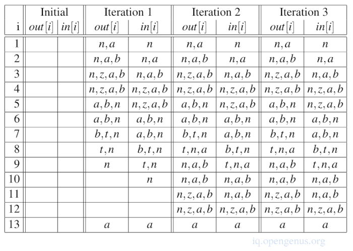
In and out sets are initialized as empty sets and iteration happens until a fixed point is reached.
The order in which we treat instructions will determine how quickly we reach the fixed-point but has no effect on the final result of the iteration.
Information in the describe equations flows backwards therefore we calculate out[i] before in[i].
In the above example each iteration calculates sets in the following order.
out[13], in[13], out[12], in[12], ... , out[1], in[1].
The most recent values are used when calculating the right sides of the equations and therefore when a value comes from a higher instruction number, the value from the same column is used.
By the 3rd iteration we have reached a fixed point a the results stop changing after the second iteration.
Interference.
Below we have a fixed-point iteration for a liveness analysis, we shall use it to explain the concept of interference.
Definition: A variable x interferes with a variable y if x != y and there exists an instruction i such that x ∈ kill[i], y ∈ out[i] and instruction i is not x := y.
Two variables share a register if neither interferes with another.
We can also say that two variables should not be live at the same time with the following differences.
- After x := y, x and y may be live simultaneously, but since they contain the same value they share a register. This is an optimization.
- Another case is that x is not in out[i] even if it is in kill[i] meaning we have assigned x to a value that won't be read from x. In this case x is not live after instruction i but interferes with y in out[i].
This interference will prevent an assignment to x overwriting y and is important to for preserving correctness.
The image below is an interference graph for the Nth fibonacci program
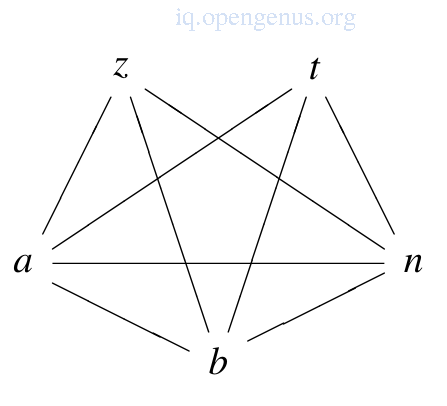
It is an undirected graph whereby each node is a variable and there is an edge between nodes x and y if x interferes with y or vice versa.
We generate interference for each assignment statement using the definition above
| Instruction | Left Side | Right Side |
|---|---|---|
| 1 | a | n |
| 2 | b | n, a |
| 3 | z | n, a, b |
| 7 | t | b, n |
| 8 | a | t, n |
| 9 | b | n, a |
| 10 | n | a, b |
| 11 | z | n, a, b |
For register allocation, two variables interfere if they also interfere at any point in the program, interference can also define a symmetric relationship between variables since two involved variables cannot share a register.
A variable cannot interfere with itself and therefore the relation is not reflective.
Register Allocation by graph coloring.
Two variables share a register if they are not connected by an edge in the interference graph.
For this we assign to each node in the interference graph a register number such that:
- Two nodes sharing an edge will have different numbers.
- The total number of different registers is less than or equal to the number of available registers.
This is known as graph-coloring(where color = register).
This problem is an NP-complete problem and therefore we need heuristic methods to find solutions where in some cases if a solution doesn't exists the method will give up.
The idea of this heuristic method is as follows; If a node in the graph has strictly fewer N edges, where N is the number of available colors(registers), we set the node aside and color the rest of the graph.
After coloring is done, nodes(n-1) connected by edges to the selected node cannot possibly use all N colors therefore we can pick a color for the selected node from the remaining colors.
Coloring the graph from the previous section is as follows
- z has three edges (3 < 4), we remove z from the graph.
- a has less than four edges, we remove a from graph.
- With the three nodes(b, t, n) left, we give each of them a number e.g 1, 2, 3 respectively.
- The three nodes(b, t, n) are connected to a, and they use three colors(1, 2, 3), we select a fourth color, e.g 4.
- z is connected to a, b, n therefore we choose a color different from 1, 3, 4 which gives 2, which works.
Algorithm.
- Initialize an empty stack.
Simplification - If there exists a node with less than N edges, place it on the stack along with a list of nodes connected to it and remove it and its edges from the graph.
2.1 If there is a node with less than N edges, select any node and repeat the above step.
2.2 If there are more nodes left in the graph, continue simplifying otherwise start selection.
Selection
3. Take a node and its connected nodes from stack an give a color different from other colors of the connected nodes.
3.1. If this is not possible, the coloring fails and we mark it for spilling
3.2. If there are more nodes in the stack process the with selection.
Points unspecified in the algorithm.
From simplification: Node to choose when none of them have less than N edges.
From Selection: Color to choose if there exists several choices.
If both of the above are chosen correctly we have an optimal coloring algorithm, unfortunately computing these choices is costly and therefore we opt to make qualified guesses.
We shall see how this can be done in the heuristics section.
Spilling.
If the selection phase is unable to find a color for a node the the graph-coloring algorithm fails meaning we give up keeping all variables in registers and hence select some variables which will reside in memory. This is spilling.
When we choose variables for spilling, we change the program so that they are kept in memory.
For each spilled variable x:
- We choose a memory address.
- In every instruction i that reads or assigns x, we rename x to xi.
- We insert instruction xi to M[addressx] before the instruction i reads xi.
- After the instruction i that assigns xi, we insert instruction to M[addressx] := xi.
- If x is live at the start of the program, we add the instruction M[addressx] := x to the start of the program.
- If x is live at the end of the program we add instruction x := M[addressx] to the end of the program.
In steps 5 and 6, we use the original name for x.
Following the above, we perform register allocation again.
Additional subsequent register allocations may generate additional spilled variables for the following reasons:
- We ignore spilled variables when selecting colors for a node in the selection phase.
- We change choices for nodes to remove from the graph in the simplification and selection phase.
Applying the algorithm to the interference graph.
| Node | Neighbors | Color |
|---|---|---|
| n | 1 | |
| t | n | 2 |
| b | t, n | 3 |
| a | b, n, t | spill |
| z | a, b, n | 2 |
Heuristics.
- Removing redundant moves.
An assignment i the form of x := y can be removed from the code if x and y use the same register because the instruction will have no effect.
Most registers will try to allocate x and y in the same register whenever possible so as to remove such redundant move instructions.
Assuming x has been assigned a color at the time we need to select a color for y, we choose the same color for y if it is not used by any variable that y interferes with(including x).
Similarly if x is uncolored, we give it the same color as y if the color is not used for a variable that interferes with x.
This is called biased coloring.
We can also combine x and y into a single node before coloring the graph and only split the combined node if the simplification cannot find a node with less than N edges. This is called coalescing.
We can also perform live-range-splitting a converse of coalescing where by instead of splitting a variable we split its node by giving each occurrence of the variable a different name and inserting assignments between them when necessary.
- Use of explicit register numbers.
Some operations require arguments or results stored in specific registers e.g integer multiplication in X86 processors require the first argument to be in the eax register and places the 64-bit result in the eax and edx registers, 32-bits each.
Variables to such operations must be assigned to these registers before register allocation begins. These are pre-colored nodes in the interference graph.
If two pre-colored nodes interfere we cannot make a legal coloring of the graph, a costly solution would be to spill one or both.
An optimal solution is to insert move instructions to move variables to and from the required registers before and after an instruction that requires specific registers.
This specific register must be included as pre-colored nodes in the interference graph but are not removed from it in the simplification phase.
Once pre-colored nodes remain in the graph, the selection phase will begin and when it needs to color a node, it avoids colors used by other neighbors to the node whether pre-colored or colored in the selection phase.
The register allocator removes the inserted moves using the methods described heuristic 1.
Summary.
Although scheduling and selection of registers assume infinite number of registers, processors only have a limited number of registers
Register allocation is the mapping of a large number of variables into a limited number of registers.
Register allocation aims to minimize space used for spilled values.
Register allocation aims to use fewer registers and minimize loads and stores.
References.
- Register Allocation Slides (PDF) by Hugh Leather from University of Edinburgh.
- "Basics of Compiler Design" by Torben Ægidius Mogensen Chapter 9.