Machine independent Optimizations

Code written in high-level programming languages has a lot of overhead, in this article we discuss low-level techniques used to optimize this code for efficiency.

Table of contents.

1. Introduction.
2. Sources of optimizations.
3. Semantic preserving optimizations.
4. Summary.
5. References.

Introduction.

Source code written in high level languages presents a lot of overhead, that is, if we translate each construct into machine code in a naive manner.
In this article, we shall see ways in which we eliminate such inefficiencies. This process of eliminating unnecessary code or replacing instructions so as to achieve better results in terms of performance is referred to as code optimization.

Optimizations are mostly based in data-flow analyses - algorithms that collect information about the program.

Sources of optimizations.

After code is optimized by the compiler it is required that its semantics be preserved, except in special circumstances e.g, when a programmer uses an algorithm that the compiler cannot understand enough about in order to replace it with a more efficient one. This is because the compiler only knows what to do with low-level semantic transformations using general facts.

Redundancy.

Redundant operations are common in programs for example an unnecessary recalculation, in such cases it is the responsibility of the compiler to spot such redundancy and eliminate it to make the code more efficient. In most cases, redundancy comes about from using high level languages and in most cases programmers are not aware of these redundancies and hence cannot eliminate them.

Semantics-preserving code optimizations.

Some of the ways a compiler can optimize source code while preserving the semantics are; common sub-expression elimination, copy propagation, dead-code elimination and constant folding

An example: Quicksort

void quickSort(int m, int n){
	int i, j;
	int v, x;
	if(n <= m) return;
	// fragment
	i = m - 1; j = n; v = a[n];
	while(1){
		do i = i + 1; while(a[i] < v);
		do j = j - 1; while(a[j[ > v);
		if(i >= j) break;
		// swap
		x = a[i]; a[i] = a[j]; a[j] = x;
	}
	// swap
	x = a[i]; a[i] = a[n]; a[n] = x;
	// end fragment
	quickSort(m, j); quickSort(i+1, n);
}

The program is then broken down to low-level arithmetic operations so as to expose redundancies.
Here we assume integers take up four bytes.
The three-address code for quicksort would resemble the following;
[image - 1]

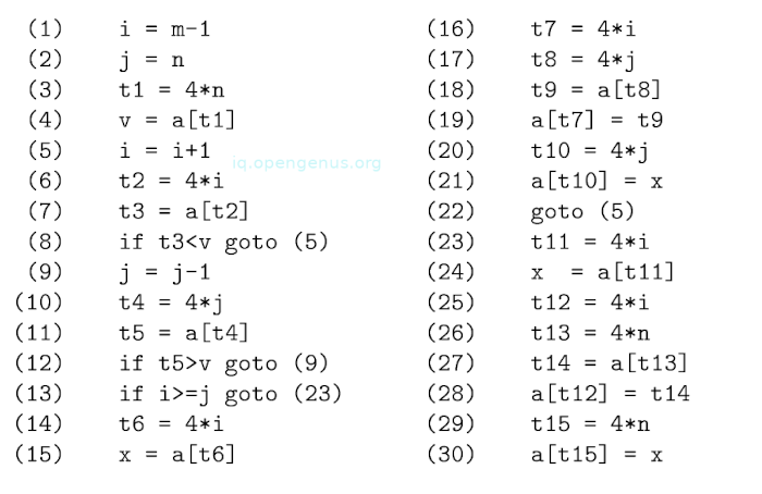
The assignment x = a[i] - from the code, is translated into two three-address statements as shown from the above image, (14), (15);
t6 = 4 * i
x = a[t6]

In a similar manner a[j] = x is also translated into two statements, (20) and (12);
t10 = 4 * j
a[t10] = x

Every array access is translated into a pair of steps and as a result we have a long sequence of three-address operations.

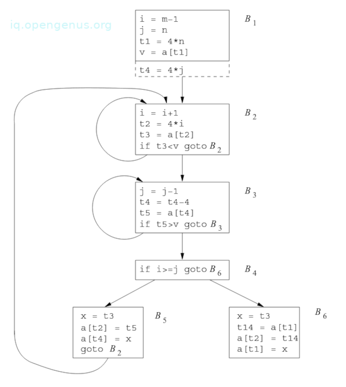
The flow-graph of the quicksort program fragment is shown below;
[image 2]

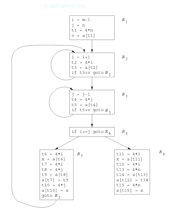
From the image, block B1 is the entry node. Conditional and unconditional jumps to statements in the three-address code are replaced in the flow graph by jump to the block of which the statements are leaders.
From the flow graph we see three loops, the blocks B2 and B3 are both loops and blocks, B2, B3, B4, B5 together form the third loops, B2 is the entry point of the loop.

As we have stated earlier, duplications such as calculations of the same value cannot be avoided by a programmer since they lie below the level of detail accessible within the source code. An example is shown below;
[image 3]

Block B% from above recalculates 4 * i and 4 * j. These calculations are however not explicitly requested by the programmer.

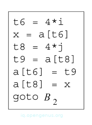
Now after local common-subexpression elimination we have a new Block 5.
[image 4]

Common global sub-expressions.

An occurrence of an expression E is referred to as a common sub-expression if it was previously computed and its values remain unchanged. In optimizations we aim to avoid such re-computations.

From the previous example above, the assignments t7 and t10 compute common subexpressions, notice that these steps have been eliminated in [image 4] where by t6 is used instead of t7 and t8 instead of t10.

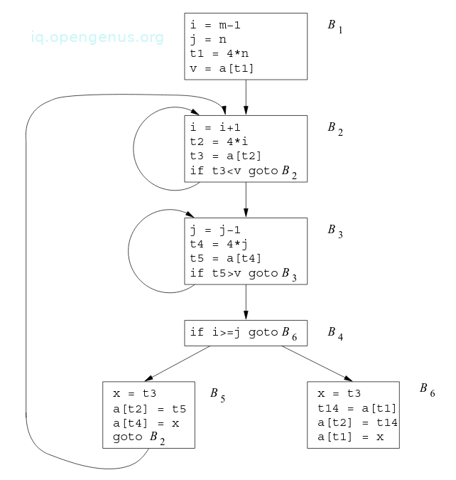
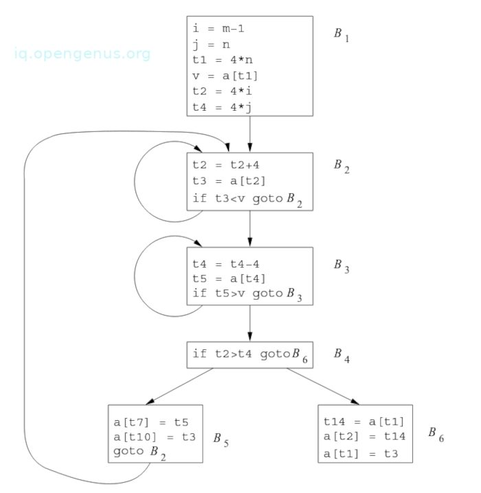
Now to eliminate both local and global common subexpressions from blocks B5 and B6 in the flow graph.
[image 5]

After local common subexpressions are eliminated, B5 still evaluates 4 * i and 4 * j as can be seen from the image. Both are common subexpressions, especially the three statements;
t8 = 4 * j
t9 = a[t8]
a[t8] = x

Which are replaced by;
t9 = a[t4]
a[t4] = x

by using t4 that is computed in block B3.

From [image 5] notice that as control passes from the evaluation of 4 * j n B3 to B5, j and t4 don't change and therefore t4 can be used when 4 * j is needed.

Another common subexpression is in block B5 after t4 replaces t8. The new expression corresponds to a[j]'s value at the source level. Not only does j retain its value when control leaves Block B3 to enter B5 but a[j] - a value computed into t5 does too and since there aren't any assignments to elements of the array a in the interim, the statements;
t9 = a[t4]
a[t6] = t9
in B5 are replaced by
a[t6] = t5

It is clear that the value assigned to x in block B5 in the [image 4] is seen to be similar to the value assigned to t3 in block B2.
Block B5 in [image 4] comes as a result of eliminating common subexpressions that correspond to the values of the source level expressions a[i] and a[j] from block B6 in [image 4].

A similar series of transformations is also performed to B6 in [image 5]

Expression a[t1] in blocks B1 and B6 in [image 4] is not a common subexpression, although t1 can be used in both blocks.
When control leaves B1 and before it reaches B6, it goes through B5 where there are assignments to a and therefore a[t1] will not have the same vale when it reaches B6 and thus it is not safe to treat a[t1] as a common subexpression.

Copy propagation.

Block B5 is further improved by the elimination of x using two new transformations. The first concerns assignments in the form of u = v referred to as copy statements/copies.
Algorithms including those for eliminating common subexpressions introduce copies.
[image 6]

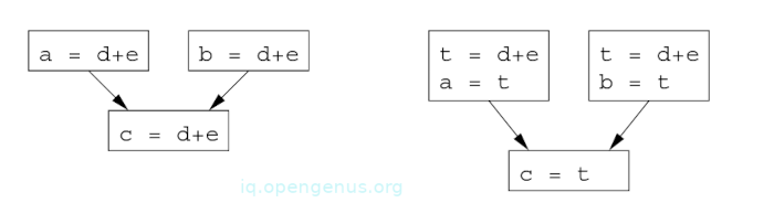
An example:
From the image above, in order to eliminate the common subexpression from statement c = d + e, we use a new variable t that holds the value d+e. This value is then assigned to c. Since control may reach c = d+e after the assignment to a or after the assignment to b, it would be incorrect to replace c = d+a with either c = a or with c = b

Copy propagation involves using v for u wherever possible after the copy statement u = v.
E.g, the assignment x = t3 in Block B5 in [image 5] is a copy, when copy propagation is applied, B5 yields the following code:
[code 1]
x = t3
a[t2] = t5
a[t4] = t3
goto B2

This may not seem as an improvement but as we shall come to see in the following section involving dead code elimination, it gives us an opportunity to eliminate the assignment to x.

Dead code elimination.

In a program, if a variable can be subsequently used, we call it live otherwise it is referred to as dead.
Dead code are statements that compute values that are never used. Dead code may come as a result of previous transformations.

An example:
We assume debug is set to TRUE or FALSE at different points in the program and used in statements for example;
if(debug) action...
It is possible for the compiler to deduce each time the program reaches this statement that the value of debug is FALSE, if there is a statement;
debug = FALSE
that must be the last assignment to debug before any tests of the value of debug.
If copy propagation replaces debug with FALSE, the action is deemed dead since it cannot be reached.
We eliminate both the test and action from the object code. Deducing at compile time that the value of an expression is a constant and using the constant instead is referred to as constant folding.

An advantage of copy propagation is that, often it turns the copy statement into dead code. E.g, copy propagation followed by dead code elimination removes the assignment to x and transforms the code in [code 1] to
a[t2] = t5
a[t4] = t3
goto B2

This is further improvement of block B5 in [image 5].

Code motion.

Loops are a key part in optimizations, especially inner loops where a program will spend most of its time.
The run time of a program is improved if we decrease the number of instructions in an inner loop even if we increase the code outside the loop.
Code motion is an important optimization that decreases the amount of code inside a loop., it takes an expression that yields the same results independent of the number of times a loop is executed and evaluates it before the loop.

An example:
An evaluation of limit-2 is a loop-invariant computation in the following while statement;
while(i <= limit-2)

Code motion produces the following code;
t = limit-2
while(i <= t)

Now, the computation of limit-2 is only performed once, before we enter the loop.
Before there would be n+1 calculations of limit-2 if we iterated the loop body n times.

Induction variables and strength reduction.

This optimization technique involves finding induction variables in loops and optimizing their computation.
A variable x is said to be an induction variable if there exists a positive or negative constant c such that each time x is assigned, its value increases by c.
For example, in [image 5], i and t2 are induction variables in the loop containing b2. Induction variables are computed with a single increment(addition/subtraction) per loop iteration.
The transformation of replacing an expensive operation e.g multiplication with a cheaper one eg; addition is referred to as strength reduction.
Induction variables not only allow us to to perform strength reduction but also eliminate all but one group of induction variables whose values remain in lock step as we go around the loop.

When loops are being processes, it is wise to work inside out, that is, start with inner loops and proceed progressively outward.
Now to see how this optimization applies to the quicksort example:
The values of j and t4 remain in lock step everytime the value of j decreases by 1, the value of t4 decreases by 4 since 4 * j is assigned to t4.
Variables j and t4 decrease by 4 thereby form an example of a pair of induction variables.

When there exists two or more induction variables in a loop, it is possible to get rid of all but one.
Looking at the inner loop of B3 in [image 5], we can't remove either j or t4 completely since t4 is used in B3 and j is used in B4.
However, we can show a reduction in strength and a part of the process of induction-variable elimination.
Eventually j is eliminated when the outer loop is considered.

An example of strength reduction applied to 4 * j in block B3
[image 7]

An example:
The relationship t4 = 4 * j holds after the assignment to t4 in [image 5] and t4 is not changed elsewhere.
It follows that after the statement j = j - 1 the relationship t4 = 4 * j + 4 must hold. We therefore replace the assignment t4 = 4 * j with t4 = t4 - 4.
The issue is that t4 doesn't have an value when we enter block B3 the first time.
Because we must maintain the relationship t4 - 4 * j on entry to the block B3, we place an initialization of T4 at the end of the block where j is initialized, this is shown by the dashed addition to block B1 in the image above;

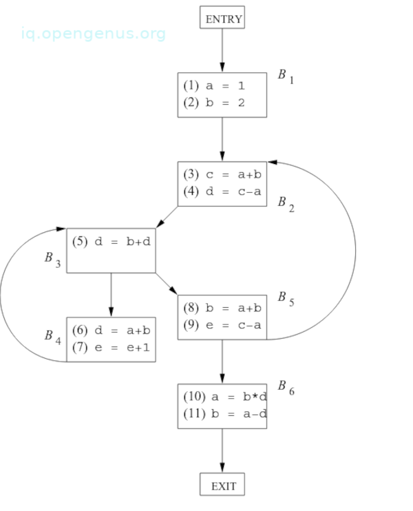
The flow graph after induction-variable elimination.
[image 8]

Although we added one more instruction that is executed one in block B1, the replacement of a multiplication with a subtraction speeds up the object code if the former takes more time than the latter.

This example treats i and j in the context of the outer loop that contains B1, B3, B4, B5.

An example:
After strength reduction is applied to the inner loops surrounding B2 and B3, the remaining use of i and j is to determine the outcome of the test in block B4.
We know the values of i and t2 satisfy the relationship t2 = 4 * i and the values of j and t4 satisfy the relationship t4 = 4 * j.
Therefore the test t2 >= t4 substitutes i >= j and when this replacement is made, i in block B2 and j in block B3 become dead variables and their assignments become dead code that is eliminated.
The resulting flow graph is seen below:
[image 9]

In [image 8], the number of instructions in blocks B2 and B2 reduce from 4 to 3 compared with the original flow graph in [image 2].
In block B5, the instructions reduce from 9 to 3 and in block B6, they reduce from 8 to 3.
In block B1, they increase from 4 to 6 however B1 is executed once therefore the total running time is not affected by its size.

Summary.

Global common subexpression finds computations of similar expressions in to basic blocks, if one precedes the other we store the result the first time and use this result for subsequent calculations.
Copy propagation is whereby a copy statement u = v assigns a variable v to a variable u, in other circumstances we replace all uses of u by v and eliminate both u and the assignment.
Code motion involves moving computations outside the loop in which it appear.
Induction variables are variables that take a linear sequence of values each time around the loop, some are used only to count iterations, oftenly we eliminate these to reduce run time.

References.

1. Compilers Principles, Techniques, & Tools, Alfred V. Aho, Monica S. Lam, Ravi Sethi, Jeffrey D. Ullman.