
Open-Source Internship opportunity by OpenGenus for programmers. Apply now.
Table of Contents
- Intoduction
- Approaches
- Brute Force
- Cell Lists
- K-D Trees
- Comparison
- Overiew
Introduction
In this article, we will be tackling the fixed radius nearest neighbor problem, this is a variation on a nearest neighbor search. Generally, we can state the problem as such: Given an input set of points in d-dimensional Euclidean space and a fixed distance Δ. Design a data structure that given a query point q, find the points of the data structure that are within distance Δ to point q.
The problem appears in fields such as molecular structure, hydrodynamics, point cloud problems and of course, computational geometry.
Approaches
There are many different approaches computer scientists have used to try and solve this problem such as brute force, cellular techniques (cell lists) and k-dimensional trees. We shall cover these techniques in the article, comparing each's performance in comparison to each other.
The fixed-radius nearest neighbour problem is a perfect example of how the GPU can be used to increase algorithm performance through parallel computing since at a large-scale, there would be many points and hence similar calculations would have to be carried out on a large amount of the same data. By utilising the many threads which GPUs contain, we can perform these calculations simultaneously instead of serially.
Brute Force
The brute force approach can be seen the same as the symetric all close pairs algorithm. It is simple in design:
- Iterate all through all the point pairs
- Compare them against distance value
- Return all points which fit this condition
The time complexity for this approach is O(n^2) and therefore is not ideal for larger scale scenarios.
@inline function distance_condition(p1::Vector{T}, p2::Vector{T}, r::T) where T <: AbstractFloat
    sum(@. (p1 - p2)^2) ≤ r^2
end

function brute_force(p::Array{T, 2}, r::T) where T <: AbstractFloat
    ps = Vector{Tuple{Int, Int}}()
    n, d = size(p)
    for i in 1:(n-1)
        for j in (i+1):n
            if @inbounds distance_condition(p[i, :], p[j, :], r)
                push!(ps, (i, j))
            end
        end
    end
    return ps
end
Cell Lists
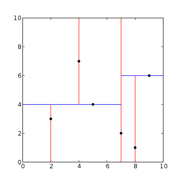
A much more efficient approach we can take is by implementing cell lists. It works on the concept of partitioning. The space we are working on is partitioned into a grid with cell size r and then associates each cell to the points that are contained by it. This method guarantees that all points within distance r are inside of a cell, or its neighbouring cells, we can refer to all point pairs as cell list pairs C. C contains all close pairs with the relationship: 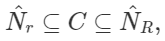 where
where  is the maximum distance between two points in neighbouring cells. We can then find the all close pairs by iteration over the cell list pairs and comparing it against the distance value.

Firstly, we can create our cell list in the code, with this mapping each cell to the indices of all the points in the cell itself.
struct CellList{d}
    indices::Dict{CartesianIndex{d}, Vector{Int}}
end

function CellList(p::Array{T, 2}, r::T, offset::Int=0) where T <: AbstractFloat
    @assert r > 0
    n, d = size(p)
    cells = @. Int(fld(p, r))
    data = Dict{CartesianIndex{d}, Vector{Int}}()
    for j in 1:n
        @inbounds cell = CartesianIndex(cells[j, :]...)
        if haskey(data, cell)
            @inbounds push!(data[cell], j + offset)
        else
            data[cell] = [j + offset]
        end
    end
    CellList{d}(data)
end
We can also define the indices to the neighbouring cells.
@inline function neighbors(d::Int)
    n = CartesianIndices((fill(-1:1, d)...,))
    return n[1:fld(length(n), 2)]
end
Next, we can say that only half of neighbouring cells have to be included since we want to avoid any duplication once iterating over the neighbours of all non-empty cells (eg. two cells could have the same neighbour). A brute force function is also written here to find all the cell list pairs by iterating over non-empty cells and finding the pairs within said cells. Then iterating over the neighbour cells checks that it is in fact, non-empty which then finds then pairs between the current cell and the non-empty one.
@inline function distance_condition(p1::Vector{T}, p2::Vector{T}, r::T) where T <: AbstractFloat
    sum(@. (p1 - p2)^2) ≤ r^2
end

@inline function brute_force!(ps::Vector{Tuple{Int, Int}}, is::Vector{Int}, p::Array{T, 2}, r::T) where T <: AbstractFloat
    for (k, i) in enumerate(is[1:(end-1)])
        for j in is[(k+1):end]
            if @inbounds distance_condition(p[i, :], p[j, :], r)
                push!(ps, (i, j))
            end
        end
    end
end

@inline function brute_force!(ps::Vector{Tuple{Int, Int}}, is::Vector{Int}, js::Vector{Int}, p::Array{T, 2}, r::T) where T <: AbstractFloat
    for i in is
        for j in js
            if @inbounds distance_condition(p[i, :], p[j, :], r)
                push!(ps, (i, j))
            end
        end
    end
end
Finding the nearest neighbours is then a case of implementing the above steps to get a solution.
function near_neighbors(c::CellList{d}, p::Array{T, 2}, r::T) where d where T <: AbstractFloat
    ps = Vector{Tuple{Int, Int}}()
    offsets = neighbors(d)
    # Iterate over non-empty cells
    for (cell, is) in c.data
        # Pairs of points within the cell
        brute_force!(ps, is, p, r)
        # Pairs of points with non-empty neighboring cells
        for offset in offsets
            neigh_cell = cell + offset
            if haskey(c.data, neigh_cell)
                @inbounds js = c.data[neigh_cell]
                brute_force!(ps, is, js, p, r)
            end
        end
    end
    return ps
end
K-D Trees
The final method we shall look at in this case is through the use of K-D trees to complete this problem. A K-D tree is an efficient data structure that again uses paritioning to more efficiently search within a given area. We can view a K-D tree as a binary tree with extra constraints on it.
We can use it to store our points in a k-dimensional space. The leaves store the points of the dataset. Each point is stored in an indiviual leaf and each leaf stores at least one point.
The time complexities of K-D tree operations can be summed as:
- Building tree ~ O(NlogN)
- Nearest neighbour search ~ O(logN)
- M nearest neighbours ~ O(MlogN)
This makes it much more efficient than our brute force approach and therefore is viable to solve this problem in general. Below is a C++ implementation of this search, using the point cloud library to generate our points.
#include <pcl/point_cloud.h>
#include <pcl/kdtree/kdtree_flann.h>

#include <iostream>
#include <vector>
#include <ctime>

int
main ()
{
  srand (time (NULL));

  pcl::PointCloud<pcl::PointXYZ>::Ptr cloud (new pcl::PointCloud<pcl::PointXYZ>);

  cloud->width = 1000;
  cloud->height = 1;
  cloud->points.resize (cloud->width * cloud->height);

  for (std::size_t i = 0; i < cloud->size (); ++i)
  {
    (*cloud)[i].x = 1024.0f * rand () / (RAND_MAX + 1.0f);
    (*cloud)[i].y = 1024.0f * rand () / (RAND_MAX + 1.0f);
    (*cloud)[i].z = 1024.0f * rand () / (RAND_MAX + 1.0f);
  }

  pcl::KdTreeFLANN<pcl::PointXYZ> kdtree;

  kdtree.setInputCloud (cloud);

  pcl::PointXYZ searchPoint;

  searchPoint.x = 1024.0f * rand () / (RAND_MAX + 1.0f);
  searchPoint.y = 1024.0f * rand () / (RAND_MAX + 1.0f);
  searchPoint.z = 1024.0f * rand () / (RAND_MAX + 1.0f);

  int K = 10;

  std::vector<int> pointIdxKNNSearch(K);
  std::vector<float> pointKNNSquaredDistance(K);

  std::cout << "K nearest neighbor search at (" << searchPoint.x
            << " " << searchPoint.y
            << " " << searchPoint.z
            << ") with K=" << K << std::endl;

  if ( kdtree.nearestKSearch (searchPoint, K, pointIdxKNNSearch, pointKNNSquaredDistance) > 0 )
  {
    for (std::size_t i = 0; i < pointIdxKNNSearch.size (); ++i)
      std::cout << "    "  <<   (*cloud)[ pointIdxKNNSearch[i] ].x
                << " " << (*cloud)[ pointIdxKNNSearch[i] ].y
                << " " << (*cloud)[ pointIdxKNNSearch[i] ].z
                << " (squared distance: " << pointKNNSquaredDistance[i] << ")" << std::endl;
  }

  std::vector<int> pointIdxRadiusSearch;
  std::vector<float> pointRadiusSquaredDistance;

  float radius = 256.0f * rand () / (RAND_MAX + 1.0f);

  std::cout << "Neighbors within radius search at (" << searchPoint.x
            << " " << searchPoint.y
            << " " << searchPoint.z
            << ") with radius=" << radius << std::endl;


  if ( kdtree.radiusSearch (searchPoint, radius, pointIdxRadiusSearch, pointRadiusSquaredDistance) > 0 )
  {
    for (std::size_t i = 0; i < pointIdxRadiusSearch.size (); ++i)
      std::cout << "    "  <<   (*cloud)[ pointIdxRadiusSearch[i] ].x
                << " " << (*cloud)[ pointIdxRadiusSearch[i] ].y
                << " " << (*cloud)[ pointIdxRadiusSearch[i] ].z
                << " (squared distance: " << pointRadiusSquaredDistance[i] << ")" << std::endl;
  }

  return 0;
}
I shall run through each step of this code and how it works to ensure understanding. Firstly, we create a point cloud with random data using the rand() function. We then create the kd-tree and use the created point cloud as an input. The given "searchPoint" is random coordinates.
Next k is defined (10 in this case) which is the number of closest points we want to find (eg. our algorithm will find the 10 closest points to our searchPoint). Two vectors are defined which are used to find the K nearest neighbours in the search.
Here instead we can also add the defined radius that we want to search in, this means the program can carry out two tasks, either K-nearest points or points within a given radius (our case). The radius here is defined as two vectors using the squared distance to find the neighbours. The points either up to K or within the given radius will then be printed to the console.
Comparison
Brute Force - O(n^2)
Cell Lists - If fixed dimension and max density (true with practical examples), number of iterations linearly proportional to the number of points O(n)
K-D Trees - Constuction of tree: O(NlogN), Nearest neighbour: O(logN)
Overview
In this article at OpenGenus we have covered the fixed-radius nearest neighbour problem with three different approaches, including analysis of algorithm and time complexity and implentations in Julia and C++. Additionally, some real-world applications have been detailed towards the start of the article, highlighting the commoness of this problem in many fields.