
Get this book -> Problems on Array: For Interviews and Competitive Programming
Reading time: 25 minutes | Coding time: 10 minutes
Bresenham Line Algorithm is a optimistic & incremental scan conversion Line Drawing Algorithm which calculates all intermediate points over the interval between start and end points, implemented entirely with integer numbers and the integer arithmetic. It only uses addition and subtraction and avoids heavy operations like multiplication and division.
Algorithm
Bresenham Line Drawing Algorithm determines the points of an n-dimensional raster that should be selected in order to form a close approximation to a straight line between two points. To draw the line we have to compute first the slope of the line form two given points.
Bresenham Line Drawing Algorithm contains two phases :
1. slope(m) < 1.
2.1 slope(m) > 1.
2.2 slope(m) = 1.
-
According to slope Decision Parameter is calculated, which is used to make decision for selection of next pixel point in both the phases.
-
Derivation of Decision Parameter Pk
* For slope(m) < 1 :
* In below figure, the y coordinate on the mathematical line at xk+1 is −
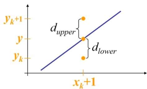
Y = m(Xk+1) + b
dupper and dlower are given as −
               dlower = y − yk
                      = m(Xk + 1) + b − Yk
               dupper = (yk + 1) − y
                      = Yk + 1 − m(Xk + 1) − b
- dupper and dlower are used to make a simple decision about which pixel is closer to the mathematical line. This simple decision is based on the difference between the two pixel positions.
- dlower − dupper = 2m(xk + 1) − 2yk + 2b − 1
- substitute m with dy/dx where dx and dy are the differences between the end-points.
           dx(dlower−dupper) = dx(2dy.dx(xk + 1) − 2yk + 2b − 1)
                             = 2dy.xk − 2dx.yk + 2dy + 2dx(2b − 1)
                             = 2dy.xk − 2dx.yk + C
- So, a decision parameter Pk for the kth step along a line is given by −
             pk = dx(dlower − dupper)
                = 2dy.xk − 2dx.yk + C
-
The sign of the decision parameter Pk is the same as that of dlower−dupper.
-
If pk is negative, choose the lower pixel, otherwise choose the upper pixel.
-
At step k+1, the decision parameter is given as −
* pk + 1 = 2dy.xk + 1 − 2dx.(yk+1) + CSubtracting pk from above statement we get −
* pk + 1 − pk = 2dy((xk+1) − xk) − 2dx((yk+1) − yk)
But, xk+1 is the same as (xk) + 1. Hence −
* pk + 1 = pk + 2dy − 2dx((yk+1) − yk)
Where, (Yk+1) – Yk is either 0 or 1 depending on the sign of Pk. -
The first decision parameter p0 is evaluated at (x0, y0) is given as −
* p0 = 2dy − dx
Similarly,
- For slope(m) > 1 && slope(m) = 1 :
- Decesion parameter -
- pk + 1 = pk + 2dx − 2dy((xk+1) − xk)
- The first decision parameter p0 is evaluated at (x0,y0) is given as −
- p0 = 2dx − dy
Pseudocode
- Step 1 : Except the two end points of Line from User.
- Step 2 : Calculate the slope(m) of the required Line.
- Step 3 : Identify the value of slope(m).
-
Step 3.1 : If slope(m) is Less than 1 i.e: m < 1
* Step 3.1.1 : Calculate the constants dx, dy, 2dy, and (2dy – 2dx) and get the first value for the decision parameter as -
* p0 = 2dy − dx
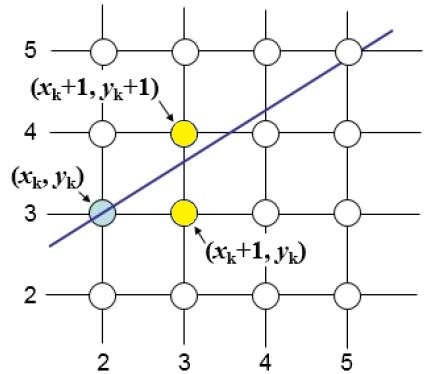
* Step 3.1.2 : At each Xk along the line, starting at k = 0, perform the following test −
* If pk < 0, the next point to plot is (xk + 1,yk) and
pk+1 = pk + 2dy
else
* plot (xk,yk + 1)
* pk+1 = pk + 2dy − 2dx
* Step 3.1.3 : Repeat step 4(dx - 1) times. -
Step 3.2 : If slope(m) is greater than or equal to 1 i.e: m >= 1
* Step 3.2.1 : Calculate the constants dx, dy, 2dy, and (2dy – 2dx) and get the first value for the decision parameter as -
* p0 = 2dx − dy
* Step 3.2.2 : At each Yk along the line, starting at k = 0, perform the following test −
* If pk < 0, the next point to plot is (xk,yk + 1) and
pk+1 = pk + 2dx
else
* plot (xk + 1,yk)
* pk+1 = pk + 2dx − 2dy
* Step 3.2.3 : Repeat step 4(dy - 1) times.
-
- Step 3.3 : Exit.
Implementation
#include <iostream>

class BresenhamLineDrawingAlgorithm
{

public:
    void bresenhamLineDrawing() const;

    void getCoordinates();

private:
    int x1_, x2_, y1_, y2_;

};

void BresenhamLineDrawingAlgorithm::bresenhamLineDrawing() const
{
    //calculating range for line between start and end point
    int dx = X2 - X1;
    int dy = Y2 - Y1;

    int x = X1;
    int y = Y1;

    //this is the case when slope(m) < 1
    if(abs(dx) > abs(dy))
    {
        putpixel(x,y,GREEN);    //this putpixel is for very first pixel of the line
        int pk = (2 * abs(dy)) - abs(dx);

        for(int i = 0; i < abs(dx) ; i++)
        {
            x = x + 1;
            if(pk < 0)
                pk = pk + (2 * abs(dy));
            else
            {
                y = y + 1;
                pk = pk + (2 * abs(dy)) - (2 * abs(dx));
            }
            putpixel(x,y,GREEN);
            delay(10);
        }
        delay(30);
    }
    else
    {
        //this is the case when slope is greater than or equal to 1  i.e: m>=1
        putpixel(x,y,GREEN);    //this putpixel is for very first pixel of the line
        int pk = (2 * abs(dx)) - abs(dy);

        for(int i = 0; i < abs(dy) ; i++)
        {
            y = y + 1;
            if(pk < 0)
                pk = pk + (2 * abs(dx));
            else
            {
                x = x + 1;
                pk = pk + (2 * abs(dx)) - (2 *abs(dy));
            }

            putpixel(x,y,GREEN);    // display pixel at coordinate (x, y)
            delay(10);
        }

        delay(30);
    }
}

void BresenhamLineDrawingAlgorithm::getCoordinates()
{
    std::cout << "\nEnter the First Coordinate ";
    std::cout << "\nEnter X1 : ";
    std::cin >> x1_;
    std::cout << "\nEnter Y1 : ";
    std::cin >> y1_;
    std::cout << "\nEnter the Second Coordinate ";
    std::cout << "\nEnter X2 : ";
    std::cin >> x2_;
    std::cout << "\nEnter Y2 : ";
    std::cin >> y2_;

}

int main()
{
    BresenhamLineDrawingAlgorithm b;
    b.getCoordinates();
    int gd=DETECT,gm;
    initgraph(&gd,&gm,NULL);
    b.bresenhamLineDrawing();

}
Which line drawing algorithm is faster ?
Advantage
-
Use of only Addition and Substraction unlike heavy operations in DDA like Multiplication and Division which require special math co-processor to get good performance.
-
No required of additional hardware in Bresenham Line Drawing Algorithm.
-
No need of floor or ceil function for displayn in Bresenham Line Drawing Algorithm.
Complexity
The time and space complexity of Bresenham Line Drawing Algorithm are:
- Worst case time complexity:
Θ(n) - Average case time complexity:
Θ(n) - Best case time complexity:
Θ(n) - Space complexity:
Θ(1)
where N is the number of intermediate point between end and start points.
Further reading
For learn another Line Drawing Algorithm, read: