Understand Genetic Algorithm with overfitting example

In this article, we have explored the ideas in Genetic algorithms (like crossover, Simulated Binary Crossover, mutation, fitness and much more) in depth by going though a Genetic algorithm to reduce overfitting.

Given coefficients of features corresponding to an overfit model the task is to apply genetic algorithms in order to reduce the overfitting.

The overfit vector is as follows:

    [0.0, 
    0.1240317450077846, 
    -6.211941063144333, 
    0.04933903144709126, 
    1.0.03810848157715883, 
    2.8.132366097133624e-05, 
    3.-6.018769160916912e-05, 
    4.-1.251585565299179e-07, 
    5.3.484096383229681e-08, 
    6.4.1614924993407104e-11, 
    7.-6.732420176902565e-12]

A genetic algorithm is a search heuristic that is inspired by Charles Darwin’s theory of natural evolution.

The implementation is as follows:

• Initialize a population
• Determine fitness of population
• Until convergence repeat the following:
  • Select parents from the population
  • Crossover to generate children vectors
  • Perform mutation on new population
  • Calculate fitness for new population

Each population contains multiple individuals where each individual represents a point in search space and possible solution.

Every individual is a vector of size 11 with 11 floating point values in the range of [-10, 10].

The theoretical details of each stage are given here:

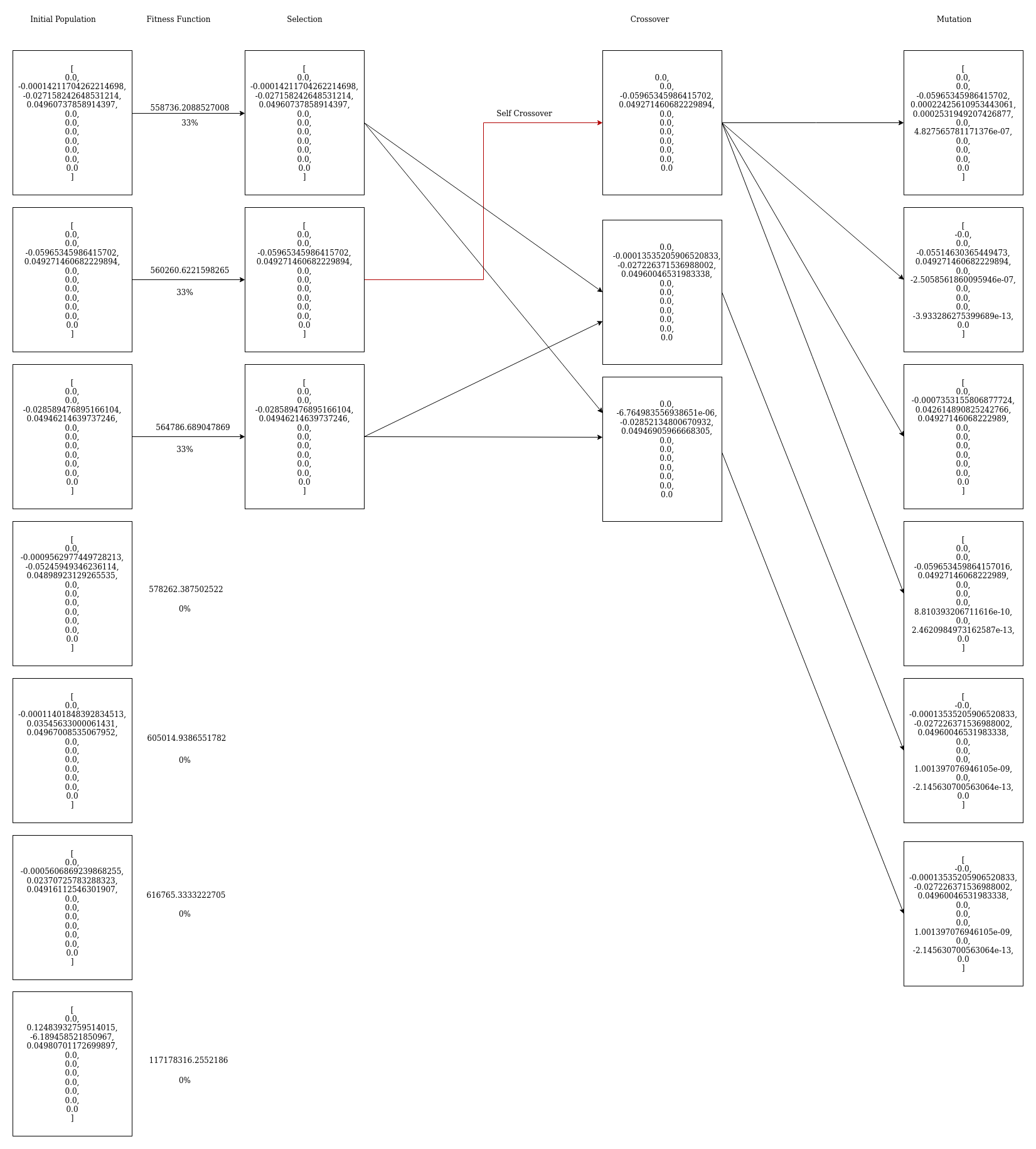
Selection

The idea is to give preference to the individuals with good fitness scores and allow them to pass there genes to the successive populations.

Crossover

This represents mating between individuals to generate new individuals. Two individuals are selected using selection operator and combined in some way to generate children individuals

Mutations

The idea is to insert random genes in offspring to maintain the diversity in population to avoid the premature convergence.

Algorithm And Code Explanation

The first population is created using an initial vector where all genes are initialized to zero. Copies of this vector are made on which I mutate to generate a population of size POPULATION_SIZE.

For each vector, at every index mutation is performed with a probability of 3/11. Then the value at that index is replaced with the value at the overfit vector at that index multiplied by some factor chosen uniformly between (0.9, 1.1).

The fitness of the population is an arithmetic combination of the train error and the validation error.

After the population is initialized, a mating pool is made (of MATING_POOL_SIZE) containing the best fitness parents.

The mating pool is selected from the population by sorting the population based on its fitness and then selecting MATING_POOL_SIZE number of vectors from the top.

def create_mating_pool(population_fitness):
    population_fitness = population_fitness[np.argsort(population_fitness[:,-1])]
    mating_pool = population_fitness[:MATING_POOL_SIZE]
    return mating_pool

Then parents are uniformly chosen from the mating pool as follows:

parent1 = mating_pool[random.randint(0, MATING_POOL_SIZE-1)]
parent2 = mating_pool[random.randint(0, MATING_POOL_SIZE-1)]

A Simulated Binary Crossover is then performed on the parents to generate an offspring.
This is followed by mutation of chromosomes, details of which are given here.

The new population is created by choosing X top children generated and POPULATION_SIZE - X top parents.

def new_generation(parents_fitness, children):
    children_fitness = calculate_fitness(children)
    parents_fitness = parents_fitness[:FROM_PARENTS]
    children_fitness = children_fitness[:(POPULATION_SIZE-FROM_PARENTS)]
    generation = np.concatenate((parents_fitness, children_fitness))
    generation = generation[np.argsort(generation[:,-1])]
    return generation

This process is repeated and the values are stored in a JSON file from which I read the next time I commence.

As you can see the code is vectorized and completely modular as separate functions have been written for each significant step.

Iteration Diagrams

First Iteration

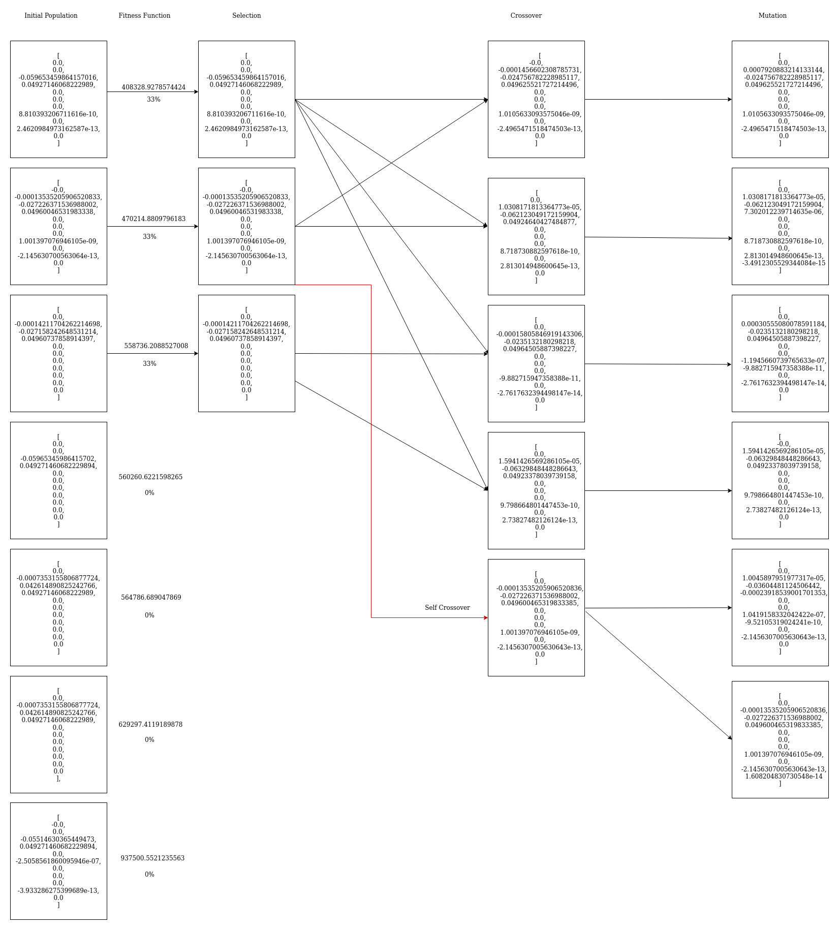
Second Iteration

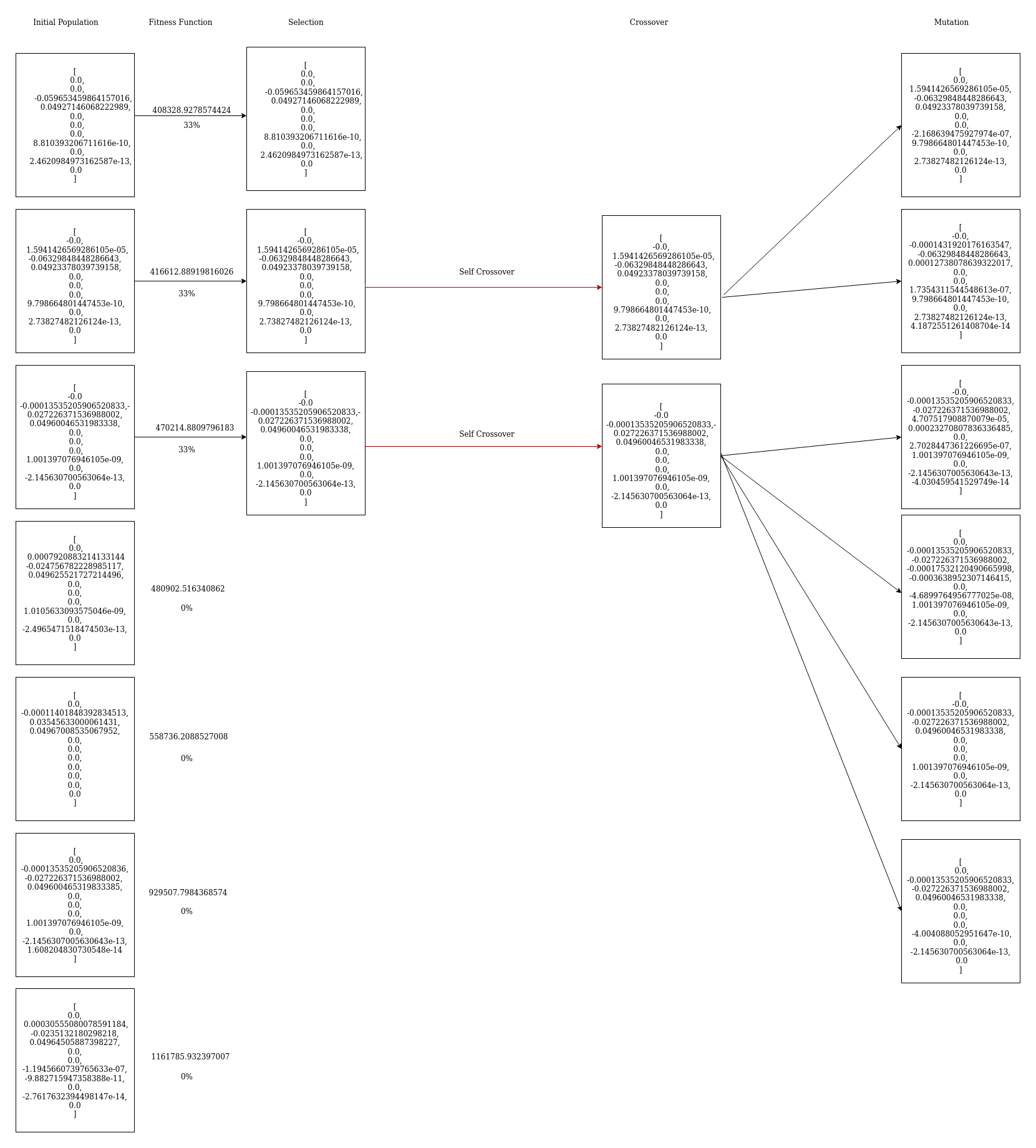
Third Iteration

Initial-Population

At first, I used the overfit vector as the initial vector to create our initial population. .

However, even after running the GA many times with different variations, I got stuck at a local minima (errors stopped improving).

So I decided to bring in some randomization in our initial vector.

I tried many things and at one point even initialized each gene of the vector with a random number between (-10, 10) . However, I soon realized that this would not work as the search space would become huge and convergence time too large.

I had to apply heuristics for our choice of initial vector

I noticed that many genes were of lower orders such as 1e-6, 1e-7.., 1e-12 and so on. Hence, I initialized all genes of the first vector to 0 during our trial and error process.

I applied mutations to this that were equivalent to some factor multiplied by the overfit vector value at that index. This would increase our probability of reaching a global minima.

Voila!
Our heuristic worked as the fitness dropped to 600K in the very first run! When I started with overfit vector, the least it reached was 1200K.

Fitness

In the fitness function, get_errors requests are sent to obtain the train error and validation error for every vector in the population.

The fitness corresponding to that vector is calculated as

absolute value of 'Train Error * Train Factor + Validation Error'

for i in range(POPULATION_SIZE):
    error = get_errors(SECRET_KEY, list(population[i]))
    fitness[i] = abs(error[0]*train_factor + error[1])

I changed the value of the train_factor from time to time, depending on what our train and validation errors were for that population. This helped us achieve a balance between the train and validation error which were very skewed in the overfit vector.I kept changing between the following 3 functions according to the requirement of the population (reason for each function mentioned below).

Train factor = 0.7

I used train_factor = 0.7 to get rid of the overfit . The initial vector had very low train error and more validation error. With our fitness function, I associated less weight to the train error and more to validation error, forcing validation error to reduce yet not allowing train error to shoot up. I also changed it to values 0.6 and 0.5 in the middle to get rid of the overfit faster. 0.7, however, worked best as it did not cause train error to rise up suddenly, unlike its lower values.

Train factor = 1

The fitness function now became a simple sum of train and validation error.

This was done when the train error became significantly large. At this point, I wanted to balance both errors and wanted them to reduce simultaneously so I set the fitness function as their simple sum.

Train factor = -1

This was done when the train error and the validation errors each had reduced greatly. However, the difference between them was still large, despite their sum being small.
So I made the fitness function the absolute difference between the train and validation error. This was done so that the errors would reach a similar value (and hence generalize well on an unseen dataset).
This function ensured the selection of vectors that showed the least variation of error between the training and validation sets.

Crossover

Single point crossover

Initially, I implemented a simple single point crossover where the first parent was copied till a certain index, and the remaining was copied from the second parent.

However, this offered very little variations as the genes were copied directly from either parent. I read research papers and found out about a better technique (described below) that I finally used.

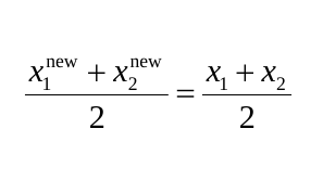
Simulated-Binary-Crossover

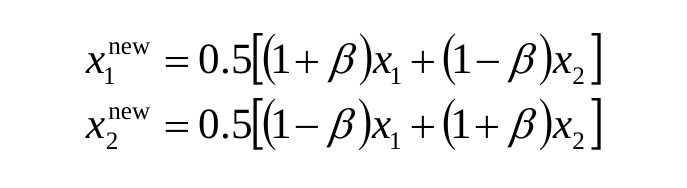
The entire idea behind simulated binary crossover is to generate two children from two parents, satisfying the following equation. All the while, being able to control the variation between the parents and children using the distribution index value.

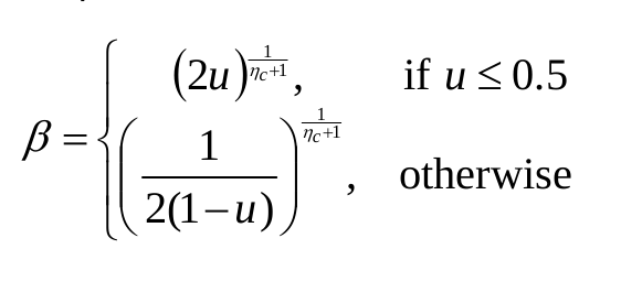
The crossover is done by choosing a random number in the range [0, 1). The distribution index is assigned its value and then $\beta$ is calculated as follows:

Distribution index that determines how far children go from parents. The greater its value the closer the children are to parents.

The distribution index is a value between [2, 5] and the offsprings are calculated as follows:

The code is as shown:

def crossover(parent1, parent2):

    child1 = np.empty(11)
    child2 = np.empty(11)

    u = random.random() 
    n_c = 3
        
    if (u < 0.5):
        beta = (2 * u)**((n_c + 1)**-1)
    else:
        beta = ((2*(1-u))**-1)**((n_c + 1)**-1)


    parent1 = np.array(parent1)
    parent2 = np.array(parent2)
    child1 = 0.5*((1 + beta) * parent1 + (1 - beta) * parent2)
    child2 = 0.5*((1 - beta) * parent1 + (1 + beta) * parent2)

    return child1, child2

I varied the Distributed Index value depending on the population.

Mutation

Our mutations are probabilistic in nature. For the vector, at every index a mutation is decided to be performed with a probability of 3/11.

I scale the value at an index by randomly choosing a value between (0.9, 1.1) iff the value after scaling is within the valid (-10, 10) range. The following code does that:

for i in range(VECTOR_SIZE):
    mutation_prob = random.randint(0, 10)
    if mutation_prob < 3:
        vary = 1 + random.uniform(-0.05, 0.05)
        rem = child[i]*vary
        if abs(rem) <= 10:
            child[i] = rem

• I chose to scale by a value close to 1 as random mutations such as setting an index to any value between (-10, 10) was not working well. I theorize this is because the overfit vector is close to good results but has just overfit on the training data. Thus, tweaking it slightly gives us improved results.

• However, I did change these mutations as per the trend of the previous populations. If I observed the errors were not reducing significantly over generations, I increased the mutations to a scaling factor between (0.9, 1.1) and even (0.3, 1.7) and other variations in tthe middle. I would experimentally observe which helped us get out of a local minima.

• Sometimes, I even decreased the mutations futher, to reach a finer granularity of our genes. I did this when I was confident I had good vectors that needed more fine tuning. I set the scaling factor between (0.997, 0.1003).

• I also applied other heuristics to it that you can read here

Hyperparameters

Population size

The POPULATION_SIZE parameter is set to 30.
We initially started out with POPULATION_SIZE = 100 as we wanted to have sufficient variations in our code. But, we realized that was slowing down the GA and wasting a lot of requests as most of the vectors in a population went unusued. We applied trial and error and found 30 to be the optimal population size where the diversity of population was still maintained.

Mating pool size

The MATING_POOL_SIZE variable is changed between values of 10 and 20.
We sort the parents by the fitness value and choose the top X (where X varies between 10 to 20 as we set it) that are selected for the mating pool.

• In case we get lucky or we observe only a few vectors of the population have a good fitness value, we decrease the mating pool size so that we can limit our children to be formed from these high fitness chromosomes. Also, when we observer that our GA is performing well and do not want unnecessary variations, we limit the mating pool size.

• When we find our vectors to be stagnating, we increase the mating pool size so that more variations are included in the population as the set of possible parents increases.

Number of parents passed down to new generation

We varied this variable from 5 to 15.

• We kept the value small when we were just starting out and were reliant on more variations in the children to get out of the overfit. We did not want to forcefully bring down more parents as that would waste a considerable size of the new population.

• When we were unsure of how our mutations and crossover were performing or when we would change their parameters, we would increase this variable to 15. We did this so that even if things go wrong, our good vectors are still retained in the new generations. This would save us the labour of manually deleting generations in case things go wrong as if there is no improvement by our changes, the best parents from above generations would still be retained and used for mating.

Distribution index (Crossover point)

This parameter was applied in the Simulated Binary Crossover. It determines how far children go from parents. The greater its value the closer the children are to parents. It varies from 2 to 5.
We changed the Distribution Index value depending on our need. When we felt our vectors were stagnating and needed variation, we changed the value to 2, so that the children would have significant variations from their parents. When we saw the errors decreasing steadily, we kept the index as 5 so that children would be similar to the parent population, and not too far away.

Mutation Range

We varied our mutation range drastically throughout the assignment.

• We made the variation as little as between factors of (0.997, 1.003) for when we had to fine tune our vectors. We did this when we were confident we had a good vector and excessive mutations were not helping. So we tried mall variations, to get its best features.

• When our vectors would stagnate and reach a local minima - we would mutate extensively to get out of the minima. The factor for multiplication could vary anywhere from (0.9, 1.1) to (0.3, 1.7).

• We would even assign random numbers at times to make drastic changes when no improvement was shown by the vectors. We did this initially when we first ran the 0 vector and it helped us achieve good results.

• Exact details as to how we did this can be found in the Mutation section.

Number of iterations to converge

Approach 1

It took 250 generations to converge when we tried with the overfit vector. The error reduced to 1.31 million total. However, we restarted after reinitializing the initial vectors as all 0s because we could not get out of this local minima.

Approach 2 (after restart)

It took 130 generations to converge. Generation 130 has validation error as 225-230K and train error around 245K for most of the vectors.

At this point the GA had converged and we had to do fine tuning to reduce the error further. It decreased very slowly after this point.
The error decreased very slowly after this point and we could finally brought the validation error down to 210K and train error to 239K.

Heuristics

• Initial vector: After almost 11 days of the assignment, our train and validation error were still at ~600K each. Initializing all genes to 0 (reason described above) reduced each error to about 300K. This was the most important heuristic we applied.

• Probabilistic mutation: Earlier we were mutating on one index only. But we changed our code to mutate each index with a probability of 3/11, this brought more variation in the genes and worked well for our populations.

• Varying mutations for different indices : We noticed as we ran our GA that the values at index 0 and 1 seemed to vary drastically, ranging much beyond what was given in the overfit vector (unlike other indices). Hence, we increased the mutations at both of these indices so as to obtain a larger search space for these. Also during our initial runs with the 0 vector and trial and error, we saw indices 5 to 11 were taking on very low values. So we kept their scaling factor between (0,1) to allow for more variations. Indices 1 to 4 had larger values in the overfit vector so we kept their scaling factor to values close to 1. These were just some modifications we kept experimenting with as we ran our code.

• Variations in fitness function, mating pool size, population size are also heuristics that we applied as the algorithm and the code could not detect when these changes were required. We had to manually study our population and see the impact of these variations and accordingly modify them.

Trace

trace.json contains the trace of the output for 10 generations.

The format is as follows,

{
    "Trace":[
    "Generation": <Generation number>,
    "Population":[[]],
    "Details":[
        "Child Number": <Index of child>,
        "Parent One:": <First parent>,
        "Parent Two:": <Second parent>
        "After Crossover": <Child generated by crossover>,
        "After Mutation": <Child after mutation>
    ]]
}

As 8 parents are brought down to new generation, the last 8 children (when sorted by fitness) are not included in the new population for the next generation.

Potential vector

• Generation: 185,

• Vector: [
  0.0,
  0.10185624018224995,
  0.004818839766729392,
  0.04465639285456346,
  -2.987380627931603e-10,
  3.817368728403525e-06,
  1.2630601687494884e-12,
  -7.311457739334194e-09,
  -2.168308617195888e-12,
  3.5200888153516045e-12,
  1.4159573224642667e-15
  ]

• Train Error: 245541.30284140716,

• Validation Error: 214556.20713485157,

• Fitness: 410989.24940797733

I believe this could be the vector on the test server as this is a vector from one of our last populations and has the best validation error I ever saw. It also has a low train error meaning it generalizes well. It is one of the vectors I submitted on the day I got the improved result.

With this article at OpenGenus, you must have a good idea of Genetic Algorithms. Enjoy.