Binary Space Partitioning Trees

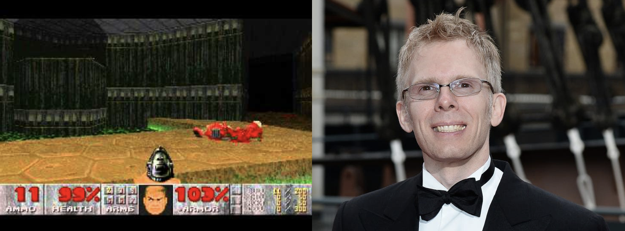
On the left is Doom, a first person shooter game was released in 1993 which then, became a phenomenon. One of the most influential games of all time.
On the right is John Carmack,a genius videoprogrammer, who ensured that the game is action-packed and frenetic!

Well, rendering a 3-D figure, isn't something particularly challenging if you have all the time in the world, but a respectable time game, needs to be swift!
He made use of Binary Space Partitioning for its agility !
Introduced in the 80s, this is a data structure of enormous potential.

As the name suggests, it refers to partitioning the space in a binary fashion, wherein it is key to be clear with what we mean by space

Space

N-dimensional space is a geometric setting in which N values (called parameters) are required to determine the position of an element (i.e., point).

Example
Two-dimensional space can be seen as a projection of the physical universe onto a plane.

What is Binary Space partitioning?

It is a method of recursively subdividing a space into two convex sets by using hyperplanes as partitions.
The resulting data structure is a binary tree, and the two subplanes are referred to as front and back.

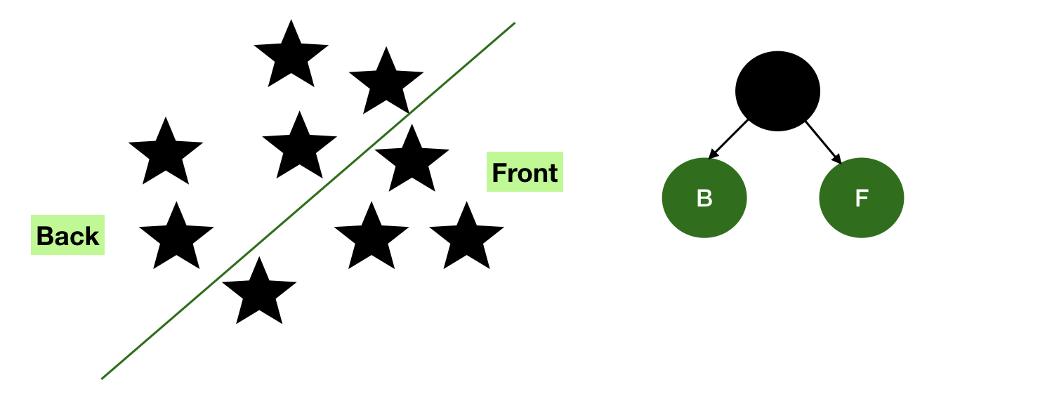
Example1

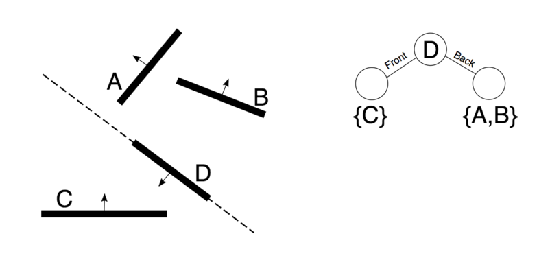
The root partitioning line is drawn along D, this splits the geometry in two sets as described in the tree.

Further spaces have been split untill no more splitting is required.

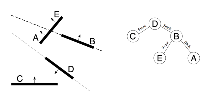
Example 2

The entire space is referred by the root node.

This is split by selecting a partition hyperplane.

These two subplanes, referred to as front and back contain more nodes, and hence shall be subdivided to get more subplanes.

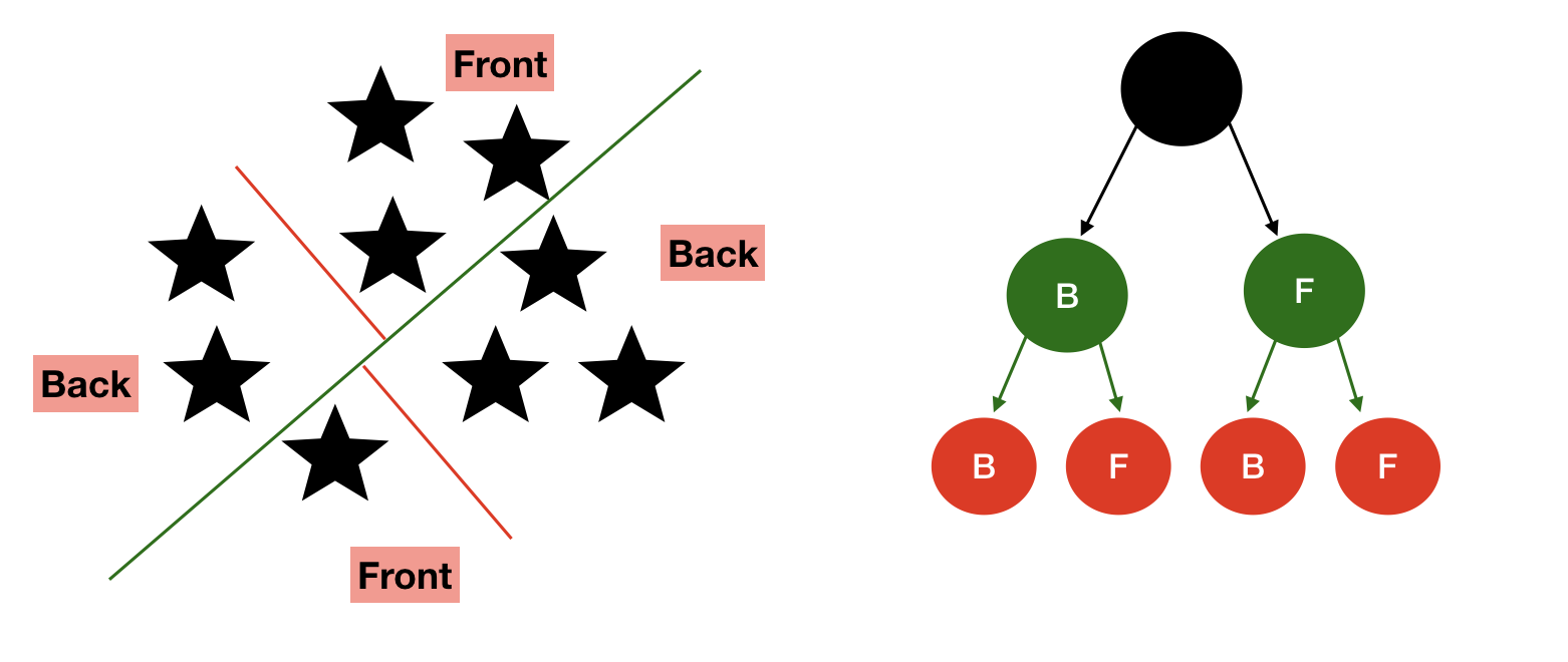
This process needs to be recursively repeated in every subspace created to finally render the complete binary tree where each leaf node contain distinct circles.

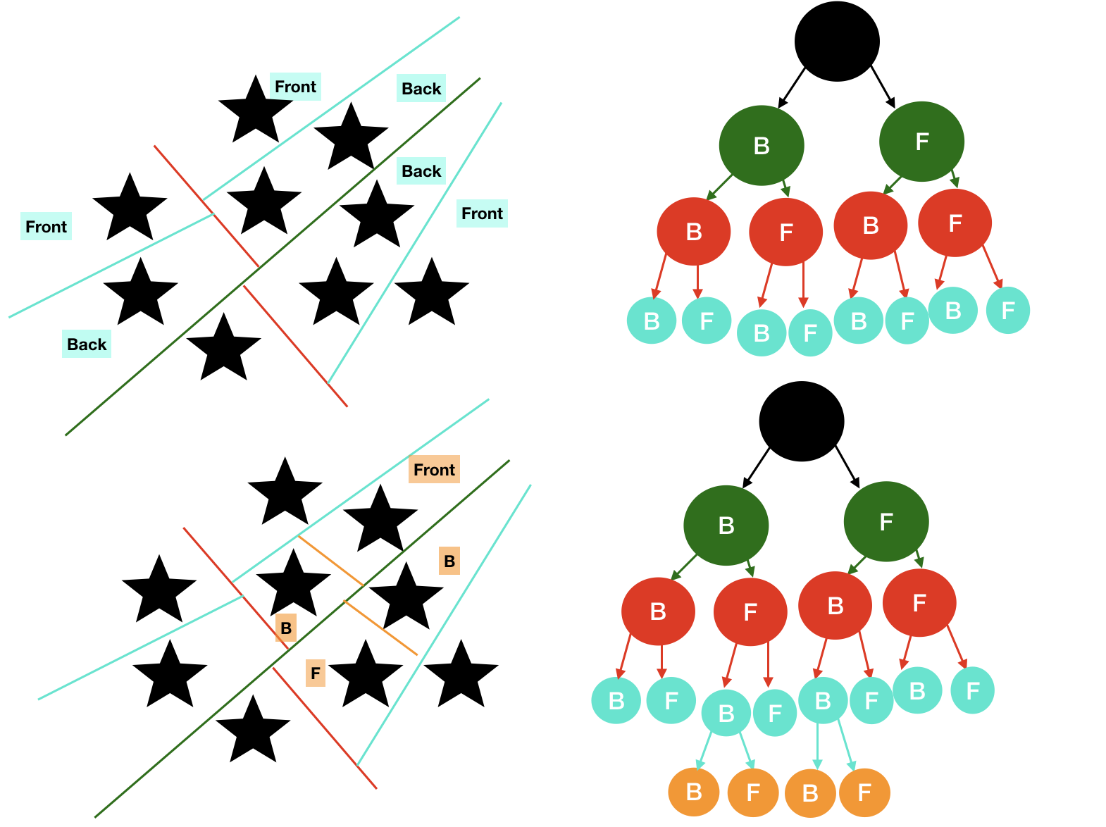
There we reach our Binary Space Partitioned Tree.

Algorithm for Common Operations

Generation

1. Choose a polygon P from the list.
2. Make a node N in the BSP tree, and add P to the list of polygons at that node.
3. For each other polygon in the list:
   • If that polygon is wholly in front of the plane containing P then: move that polygon to the list of nodes in front of P.
   • If that polygon is wholly behind the plane containing P then: move that polygon to the list of nodes behind P.
   • If that polygon is intersected by the plane containing P then: split it into two polygons and move them to the respective lists of polygons behind and in front of P.
   • If that polygon lies in the plane containing P then: add it to the list of polygons at node N.
4. Apply this algorithm to the list of polygons in front of P.
5. Apply this algorithm to the list of polygons behind P.

Time Complexity

You need to answer this question to get the time complexity.
How to bound the number of recursive calls?, Recursive calls give rise to new recursive calls (splitting), the expected number is bounded by expected number of fragments. The time complexity can be pretty fine to pretty catastrophic, depending on the space being mapped.

The time consumed for building the tree, can be compromised for quicker rendering of the tree.

Traversal

1. If the current node is a leaf node then:
   render the polygons at the current node.
2. Else if the viewing location V is in front of the current node then:
   1. Render the child BSP tree containing polygons behind the current node
   2.Render the polygons at the current node
   3.Render the child BSP tree containing polygons in front of the current node
3. Else if the viewing location V is behind the current node then:
   1.Render the child BSP tree containing polygons in front of the current node
   2. Render the polygons at the current node
   3. Render the child BSP tree containing polygons behind the current node
4. Else if the viewing location V must be exactly on the plane associated with the current node then:
   1. Render the child BSP tree containing polygons in front of the current node
   2.Render the child BSP tree containing polygons behind the current node

Time Complexity

A BSP Tree is traversed in linear time i.e. O(n), and renders the polygon in a far to near ordering, suitable for the painter's algorithm.
This ensures fast rendering i.e. the primary motive behind using Binary Space PArtitioning trees in real life situations even though generation might be costlier.

C++ Implementation

This is based on the assumption that Object exposes its position, and the Node class is responsible for, and can write on object's position.

In addition, Objects are added in the first node having room to hold it. In case all nodes are full, we create two empty children (if not done yet), each one representing half part of the parent node.

To remove an object from the tree, we have to find it. We will search it in each node recursively, using its position to take the right branch at each step. When found, we just remove it and return.

Retrieving an object from the tree is really fast when it comes to BSP Trees and the best part is, the more the depth of the tree, greater will be the efficiency in terms of data retrieval. All we have to do is to test all object in all the nodes in the interval. If a node is not in the interval, we can dismiss the entire branch in our search

class Object
{
  int pos;
public:
  int position() const;
  int & position();
};

class Node
{
  static const unsigned int depth_max = 32;
  static const unsigned int max_objects = 32;

  const unsigned int depth;
  const int min, max, center;  // geometry of node 
  std::list<Object*> objects;  // actual container for object reference
  Node *children[2];           // only constructed if actual container is full

  Node(Node const &, bool);    //Constructor to create a child 
  bool isEmpty() const;        // check if the children are empty as well
public:
  Node(int min, int max);      //Constructor to create the first node
  ~Node();                     //Destructor

  void addObject(int position, Object *);
  void delObject(Object *);
  void movObject(int newPos, Object *);

  // Get all object in requisite range 
  void getObject(int posMin, int posMax, std::list<Object*> &);
};

// Public constructor, to create root node
Node::Node(int min, int max)
: depth(0), min(min), max(max), center((min + max) / 2), objects(), children(nullptr)
{}

Node::~Node()
{
  delete[] children;
}

// Private constructor for constructing children.
// Compute it own center and range according to the side indicator.
// side specifies wich parent's side the child will represent.
Node::Node(Node const & father, bool side)
: depth(father.depth + 1),
  min(side ? father.min : father.center),
  max(side ? father.center : father.max),
  center((min + max) / 2),
  objects(),
  children(nullptr)
{}
bool Node::isEmpty() const
{
  return !((!objects.empty()) || children ||
           (children[0]->isEmpty() && children[1]->isEmpty()));
}

void Node::addObject()
{
  if (objects.size() > max_objects && depth < max_depth)
  { // if max object is reached but not depth max 
    if (!children) children = new Node(...); // create children 
    return; // pass to the corresponding child  and return 
  } // if depth max is reached and even if node is "full", execution continue 
  objects.push_back(obj); // overthrow the max_objects limit if max depth is reached 
}

void Node::delObject(Object * obj)
{
  
  if (children && children[0]->isEmpty() && children[1]->isEmpty())
    delete[] children;
    // after a deletion, if both children are empty, delete them.
}
void Node::addObject(int position, Object * obj)
{
  if (objects.size() > max_objects) // if node is full 
    if (depth < depth_max) // if we can go deeper
    {
      if (children == nullptr) // if we need to create child 
                              // we create each child corresponding to their place
        children = new { Node(*this, false), Node(*this, true) };
      // we pass the object to a child, depending on the object's position
      children[ position <= center ? 0 : 1]->addObject(position, obj);
      return; 
    }
  objects.push_back(obj); // we add in this node, in the first and last intention
  obj->position() = position; 
}

void Node::delObject(Object * obj)
{
  auto found = std::find(objects.begin(), objects.end(), obj); // find object
  if (found != objects.end()) // object found 
  {
    objects.remove(found); // removed
    return;
  }
  if (children) // check children
  {
    // recursion for corresponding children
    children[obj->position() <= center ? 0 : 1]->delObject(obj);
    if (children[0]->isEmpty() && children[1]->isEmpty())
      delete[] children; // if both children are empty, delete them
  }
}

void Node::movObject(int newPos, Object *obj)
{
  auto found = std::find(objects.begin(), objects.end(), obj); //find object
  if (found == objects.end() && children) //object not found, go deeper 
  {
    // same partition for old and new pos, recursion on the corresponding child
    if (newPos <= center && obj->position() <= center)
      children[0]->movObject(newPos, obj);
    else if (newPos > center && obj->position() > center)
      children[1]->movObject(newPos, obj);

    // remove from the old partition and add to the new one 
    else if (newPos <= center && obj->position() > center)
    {
      children[1]->delObject(obj);
      children[0]->addObject(newPos, obj);
    }
    else if (newPos > center && obj->position() <= center)
    {
      children[0]->delObject(obj);
      children[1]->addObject(newPos, obj);
    }
  }
  // object is now in the right place, so update it position
  obj->position() = newPos;
}

void Node::getObject(int posMin, int posMax, std::list<Object *> & list)
{
  // get all wanted objects in this node
  for (auto it = objects.begin(); it != objects.end(); it++)
    if (it->position() >= posMin && it->position() <= posMax)
      list.push_back(*it);

  if (childrens) // if you can, go deeper
  {
    if (posMin <= center)
      children[0]->getObject(posMin, posMax, list);
    if (posMax > center)
      children[1]->getObject(posMin, posMax, list);
  }
}

What makes this worthwhile?

Even though adding, removing, moving might be a little costlier, you may observe substantial gain at every search. As by logic, you may exclude entire branches during search which highly accelerates the process.

Searching efficiently in order to render necessary objects as quick as possible is the primary goal, in its applications.

Binary space partitioning arose from the computer graphics's need to rapidly draw three-dimensional scenes composed of polygons. A simple way to draw such scenes is the painter's algorithm. This approach has two disadvantages:

1.The time required to sort polygons in back to front order.
2. The possibility of errors in overlapping polygons was also high.

To compensate for these disadvantages, the concept of binary space partitioning tree was proposed.

Applications

Since its inception, Binary Space Partition Trees have been found to be of immense use in the following

• Computer Graphics
• Back face Culling
• Collision detection
• Ray Tracing

Game engines using BSP trees include the Doom (id Tech 1), Quake (id Tech 2 variant), GoldSrc and Source engines.

Don't forget it brought you the game that revolutionised video games!
By now you must've understood the significance, utility, concept and application of Binary Space Partition Trees.

It is your turn to revolutionise the world now!