Intermediate representations (IR) in Compiler Design

In this article, we discuss intermediate representations and look at different approaches to IR while considering their properties.

Table of contents

1. Introduction.
2. Abstract Syntax Tree(AST).
3. Directed Acyclic Graph(DAGs).
4. Control flow graph.
5. Static single assignment form.
6. Linear IR.
7. Static Machine IR.
8. Summary.
9. References.

Introduction.

Intermediate representations lie between the abstract structure of the source language and the concrete structure of the target assembly language.
These representations are designed to have simple regular structures that facilitate analysis, optimization and efficient code generation.

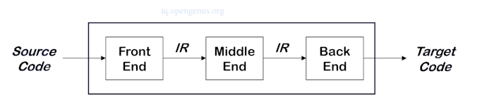
The Front-end produces the intermediate representation.
The Middle transforms the IR into a more efficient IR.
The Back-end transforms the IR into native code.

Categories of IR.

1. Structural.

• They are graphically structured.
• Used in source-to-source translators.
• Large in size.
  e.g; AST, DAGs

2. Linear.

• Simple and compact data structures.
• Easier to rearrange.
• They have a varied level of abstraction.
• They can act as pseudo-code for an abstract machine.
  e.g; 3-address code, stack machine code

3. Hybrid.

• They are a combination of graphs and linear code.
  e.g control flow graph.

Abstract syntax tree.

An AST is usable as an IR if the goal is to emit assembly language without optimizations or transformations.

An example
The AST of the expression x - 2 * y

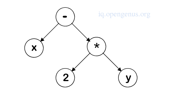
In post-fix form -> x 2 y * -
In prefix form -> - * 2 y x

After type checking, optimizations e.g constant folding, strength reduction can be applied to the AST, then post-order traversal is applied to generate assembly language whereby each node of the tree will have corresponding assembly instructions.

In a production compiler, this is not great choice for IR because the structure is too rich, in that, each node has a large number of options and substructure e.g an addition node can represent either floating point or integer addition.

This makes transformations and external representations difficult to perform.

Directed acyclic graphs.

A DAG is an AST with a unique node for each value.

A DAG can have an arbitrary graph structure whereby individual nodes are simplified so that there is little auxilliary information beyond the type and value of each node.

We have the expression x = (a + 10) * (a + 10).
The AST of the expression is shown below.

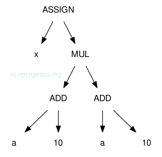
After type checking, we learn a is a floating point value so 10 must be converted to a floating point value for floating point arithmetic operation to happen.

Additionally, this computation is performed once and this result can be used twice.

The DAG for the expression.

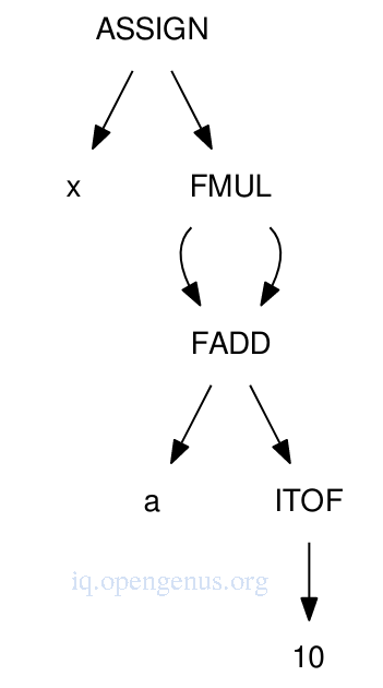
ITOF will be responsible for performing integer-to-float conversion.
FAAD and FMUL perform floating point arithmetic.

DAGs represent address computations related to pointers and arrays so that they are shareable and optimized whenever possible.
An example

An example of an array lookup for x = a[i] represented in an AST

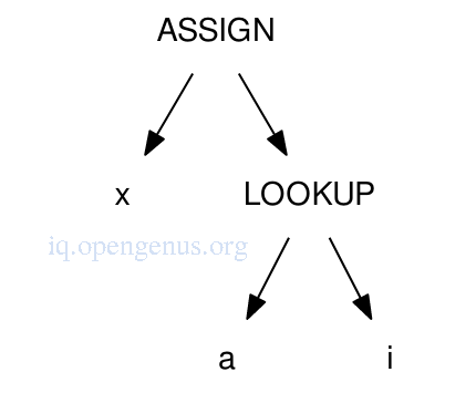
We add the starting address of array a with the index of the item i multiplied by the size of objects in the array(determined by symbol table).

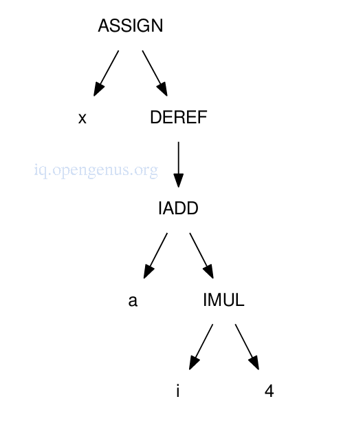
The same lookup in a DAG.

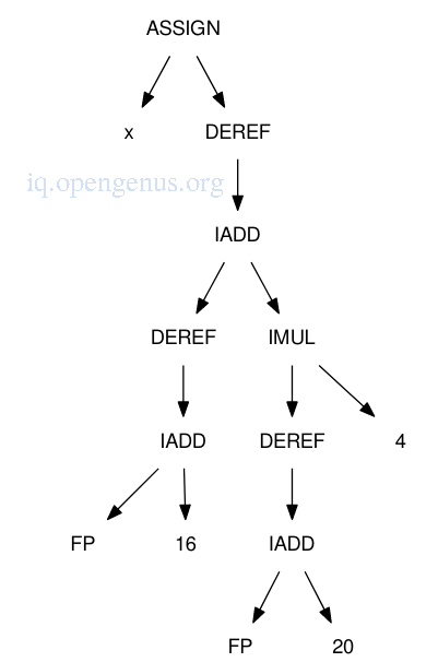
Before code generation, the DAG might be expanded so as to include address computations of local variables. e.g if a and i are both stored on the stack at 16 and 20 bytes past the frame pointer respectively, the DAG is expanded as shown below.

The value-number method can be used to construct a DAG from an AST by building an array where each entry consists of a DAG node type and array index of child nodes, such that each time we need to add a new node, we first search the array for a matching node and reuse it to avoid duplication.

By performing a post-order traversal and adding each element of the AST to an array we are able construct the DAG.

Value-number array representation of the DAG

	Type	Left	Right	Value
0	NAME			x
1	NAME			a
2	INT			10
3	ITOF	2
4	FADD	1	3
5	FMUL	4	4
6	ASSIGN	0	5

As long as each expression has its own DAG, we can avoid a polynomial complexity when searching for nodes every time there is a new addition since absolute sizes will remain relatively small.

With DAG representation it is easier to write portable external representations since all information will be encoded into a node.

To optimize a DAG we can use constant folding where by we reduce an expression consisting of constants into a single value.

Constant Folding Algorithm

The algorithm works by examining a DAG recursively and collapsing all operators with two constants into a single constant.

ConstantFold(DAGNode):
    If n is leaf:
        return;
    Else:
        n.left = ConstantFold(n.left);
        n.right = ConstantFold(n.right);
        
        If n.left and n.right are constants:
            n.value = n.operator(n.left, n.right);
            n.kind = constant;
            delete n.left and n.right;

Constant folding in practice

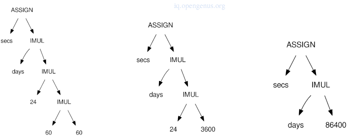
We have the expression secs = days * 24 * 60 * 60 as represented by the programmer which computes the number of seconds in the given number of days, The ConstantFold algorithm descends through the tree and combines IMUL(60, 60) to 3600 and IMUL(3600, 24) to 86400.

Control flow graph.

A DAG can encode expressions effectively but faces a drawback when it comes to ordered program structures such as controlling flow.

In a DAG common subexpressions are combined assuming they can be evaluated in any ordering and values don't change however this doesn't hold when it comes to multiple statements that modify values and control flow structures that repeat or skip statements hence a control flow graph.

A control flow graph is a directed graph whereby each node will consist of a basic block of sequential statements.

Edges in the graph represent the possible flow of control between basic blocks.
Conditional constructs e.g if or switch statements, define the branches in the graph.

Looping constructs e.g for or while loops, define reverse edges.

An example

for(i = 0; i < 10; i++){
    if(i % 2 == 0)
        print "even";
    else
        print "odd";
    print "\n";
}
return;

The control flow graph

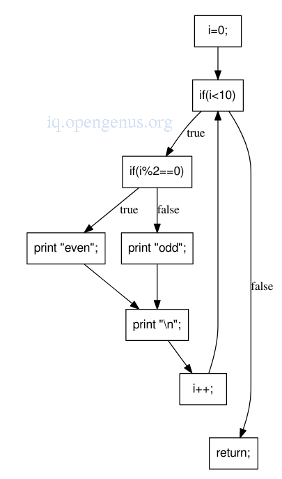
For the for loop the control flow graph places each expression in the order it would be executed in practice as compared to the AST which would have each control expression as an intermediate child of the loop node.

The if statements have edges from each branch of the conditional to the following node and thus it it easy to trace the flow of execution from a component to the next.

Static single assignment form.

The idea is to define each name exactly once.

It is a common representation for complex optimizations.

It uses information from the control flow graph and updates each basic block with a new restriction e.g variables cannot change values and when a variable indeed changes a value, it is assigned a version number.

An example
int x = 1;
int a = x;
int b = a + 10;
x = 20 * b;
x = x + 30;

In SSA
int x_1 = 1;
int a_1 = x_1;
int b_1 = a_1 + 10;
x_2 = 20 * b_1;
x_3 = x_2 + 30;

What if a variable is given a different value in two branches of a conditional? We introduce the phi ϕ-functions to make it work.

ϕ(x, y), indicates that either value x or y could be selected at run-time. This function might not translate into assembly code but serves as a link to the new value to its possible old values.

An example

if(y < 10)
    x = a;
else
    x = b;

becomes

if(y_1 < 10)
    x_2 = a;
else
    x_3 = b;
x_4 = phi(x_2, x_3);

Linear IR.

This is an ordered sequence of instructions that are closer to the final goal of an assembly language.

It looses DAG flexibility, but can capture expressions, statements and control flows within one data structure.

It looks like an idealized assembly language with a large/infinite number of registers and common arithmetic and control flow operations.

Linear IR can be easily stored considering each instruction is a fixed size 4-tuple representing the operation and arguments(max of 3).

Assume an IR with LOAD and STOR instructions to move values between memory and registers, and 3-address arithmetic operations that read two registers and write to a third from left to right.

An example expression would look like the following.

1. LOAD a        -> %r1
2. LOAD $10      -> %r2
3. ITOF %r2      -> %r3
4. FADD %r1, r3% -> %r4
5. FMUL %r4, r4  -> %r5
6. STOR %r5      -> x

We assume there exists an infinite number of virtual register so as to write each new value to a new register by which we can identify the lifetime of a value by observing the first point where a register is written and the last point where a register is used, e.g the lifetime of %r1 is from instruction 1 to 4.

At any given instruction we can observe virtual registers that are live.

1. LOAD a        -> %r1        live: %r1
2. LOAD $10      -> %r2        live: %r1 %r2
3. ITOF %r2      -> %r3        live: %r1 %r2 %r3
4. FADD %r1, r3% -> %r4        live: %r1 %r3 %r4
5. FMUL %r4, r4  -> %r5        live: %r4 %r5
6. STOR %r5      -> x          live: %r5

The above makes instruction ordering easier since any instruction can be moved to an earlier position(within on basic block) as long as the values that are read are not moved above their definitions.

Also, instructions may be moved to later positions so long as the values it writes are not moved below their uses.

In a pipelined architecture, moving of instructions reduces the number of physical registers needed for code generation and thus reduced execution time.

Stack machine IR.

This is a more compact version of IR designed to execute on a virtual stack machine without traditional registers except only a stack to hold intermediate registers.
It uses PUSH instruction to push a variable or literal onto the stack and POP instruction to remove an item from the stack and stores it in memory.

FADD and FMUL binary arithmetic operators implicitly pop two values off the stack and push the result on the stack.

ITOF unary operator pops one value off the stack and push another value.

COPY instruction manipulates the stack by pushing duplicate values onto the stack..

A post-order traversal of the AST is used so as to produce a stack machine IR given a DAG and emit a PUSH for each leaf value, an arithmetic instruction for each node and POP instruction which assigns a value to a variable.

An example expression
x=(a + 10)$*$(a + 10)

Instructions in a stack machine

PUSH a
PUSH 10
ITOF
FADD
COPY
FMUL
POP x

Assuming x is 5, executing thr IR would result in the following.

IR Operation	PUSH a	PUSH 10	ITOF	FADD	COPY	FMUL	POP x
Stack	5.0	10	10.0	15.0	15.0	225.0	-
State:	-	5.0	5.0	-	15.0	-	-

Pros of stack machine

It is much more compact compared to a 3-tuple or 4-tuple representation since there is no need for recording register details.

Implementation is straight forward in a simple interpreter.

cons.

It is difficult to translate to a conventional register-based assembly language since explicit register names are lost, further transformation and optimization requires transforming implicit information dependencies in the stack-basic IR back to a more explicit DAG or linear IR with explicit register names.

Summary.

Every compiler or language will have its own intermediate representation with some local features.

Intermediate representations are independent of the source language.
Intermediate representations express operations of a target machine.
IR code generation is not necessary since the semantic analysis phase in compiler design can generate assembly code directly.

References.

1. Constant Folding.
2. Semantic Analysis
3. Introduction to Compilers and Language Design, 2nd Edition, Prof. Douglas Thain.