
This article discusses about the YOLOv4's architecture. It outperforms the other object detection models in terms of the inference speeds. It is the ideal choice for Real-time object detection, where the input is a video stream.
Table of contents:
- Brief Introduction to Object Detection
- What is YOLOv4?
- Algorithm Overview
- Backbone Network
- Neck
- Head
- YOLOv4 Additions (Bag of Freebies and Specials)
- Results
Brief Introduction to Object Detection:
Before we proceed further, we'll understand the task of object detection.
The standard definition from Wikipedia goes like,
"Object detection is a computer technology, which is related to computer vision and image processing that deals with detecting instances of semantic objects of a certain class (like humans, buildings, cars or animals, etc.) in digital images and videos."
The task of object detection consists of two things - the first being Object Localization which is then followed by Object Classification. This is accomplished by predicting the co-ordinates of the bounding box along with the Class probabilities.
Object Detection in YOLO:
The input given is an image along with ground truth values of the bounding boxes.
The entire input image is divided into a square grid, the grid cell containing the center of the object is responsible for detecting that object. Each grid cell will predict B bounding boxes and the confidence scores associated with those boxes. This score indicates the accuracy of the box and how confident the model is that the box contains the object. Confidence score is IoU of predicted values and the ground truth values of the bounding box.
What is YOLOv4?
YOLOv4 is a SOTA (state-of-the-art) real-time Object Detection model. It was published in April 2020 by Alexey Bochkovsky; it is the 4th installment to YOLO. It achieved SOTA performance on the COCO dataset which consists of 80 different object classes.
YOLO is a one-stage detector. The One-stage method is one of the two main state-of-the-art methods used for the task of Object Detection, which prioritizes on the inference speeds. In one-stage detector models ROI (Region of Interest) is not selected, the classes and the bounding boxes for the complete image is predicted. Thus, this makes them faster than two-stage detectors. Other examples are FCOS, RetinaNet, SSD.
The first version of YOLO was written in the Darknet Framework (which is a high performance open source framework for implementing neural networks written in C and CUDA). DarkNet is typically a backbone network.
It divides the object-detection task into regression task followed by a classification task. Regression predicts classes and bounding boxes for the whole image in single run and helps to identify the object position. Classification determines the object's class.
Algorithm Overview:
The architecture consists of various parts, broadly they are - The input which comes first and it is basically what we've as our set of training images which will be fed to the network - they are processed in batches in parallel by the GPU. Next are the Backbone and the Neck which do the feature extraction and aggregation. The Detection Neck and Detection Head together can be called as the Object Detector.
And finally, the head does the detection/prediction. Mainly, the Head is responsible for the detection (both localization and classification).
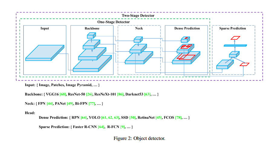
Because YOLO is a one-stage detector it does both of them simultaneously (also known as Dense Detection). Whereas, a two-stage detector does them separately and aggregates the results (Sparse Detection)
The sequence is as follows:
             Input → CSPDarknet53 → [SPP Block + PANet] → YOLOv3
                      (Backbone)          (Neck)          (Head)
YOLOv4 explores different backbone networks and data augmentation methods.
Backbone Network:
The authors initially considered CSPResNext50, CSPDarknet53 and EfficientNet-B3 as the backbone networks. Finally, after a lot of testing and experimental results they chose CSPDarknet53 CNN. (Page 7 of the paper titled "YOLOv4: Optimal Speed and Accuracy of Object Detection").
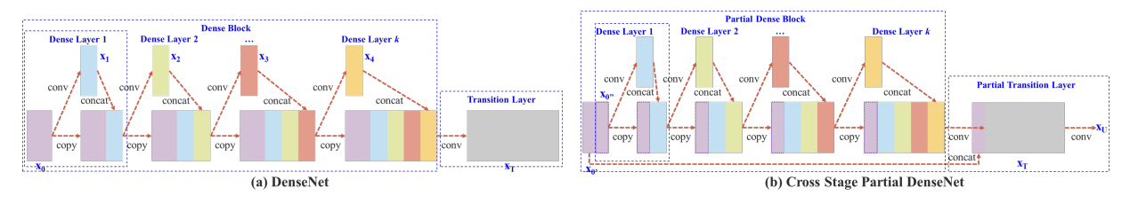
CSPDarkNet53 is based on the DenseNet design. It concatenates the previous inputs with the current input before proceeding into the dense layers - this is referred to as the Dense connectivity pattern.
CSPDarkNet53 consists of two blocks:
- Convolutional Base Layer
- Cross Stage Partial (CSP) Block
Cross Stage Partial strategy splits the feature map in the base layer into two parts and merges them with the help of Cross-stage hierarchy, this allows for more gradient to flow through the layers and thus alleviates the infamous problem of "Vanishing Gradient".
The Convolutional Base Layer consists of the full-sized input feature map.
The CSP block which is stacked next to the Convolutional Base layer, divides the input into two halves as described previously, one half will be sent through the dense block, while the other half will be routed directly to the next step without any processing. CSP preserves fine-grained features for more efficient forwarding, stimulates network to reuse features and decreases number of network parameters. Only the final convolutional block in the backbone network which is able to extract richer semantic features is a dense block as more number of densely linked convolutional layers may result in a drop in detection speed.
Neck
The neck is the part where feature aggregation takes place. It collects feature maps from the different stages of the backbone then mixes and combines them to prepare them for the next step. Usually, a neck consists of several bottom-up paths and several top-down paths.
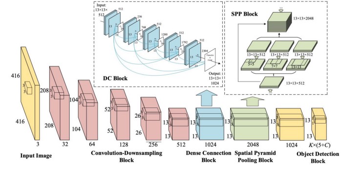
SPP - Additional Block
An additional block called SPP (Spatial Pyramid Pooling) is added in between the CSPDarkNet53 backbone and the feature aggregator network (PANet), this is done to increase the receptive field and separates out the most significant context features and has almost no effect on network operation speed. It is connected to the final layers of the densely connected convolutional layers of CSPDarkNet.
The receptive field refers to the area of the image that is exposed to one kernel or filter at an instance. As more convolutional layers are stacked, it increases linearly whereas it increases exponentially when we stack dilated convolutions and brings non-linearity.
Here's an overview of the operations performed:
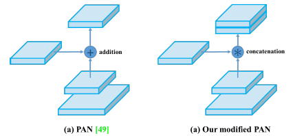
PANet (Path Aggregation Network)
YOLOv4 uses a modified path aggregation network, mainly as a design improvement in-order to make it more suitable for training on a single GPU.
The main role of PANet is to improve the process of instance segmentation by keeping the spatial information which in turn helps in proper localization of pixels for mask prediction. Bottom-up Path Augmentation, Adaptive Feature Pooling & Fully-Connected Fusion are the important properties that make them so accurate for mask prediction.
Here the modified PANet concatenates neighbouring layers instead of adding when using the Adaptive Feature Pooling.
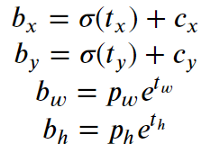
Head
The main function here is locating bounding boxes and performing classification.
The bounding box co-ordinates (x, y, height and width) as well as scores are detected. Here the x & y co-ordinates are the center of the b-box expressed relative to the boundary of the grid cell. Width & Height are predicted relative to the whole image.
How the YOLO algorithm works has been discussed in the previous section.
YOLOv4 Additions:
Two new terms were introduced by the authors called Bag of Freebies (BoF) & Bag of Specials (BoS).
Bag of Freebies (BoF): They improve performance of the network without adding to the inference time, most of which are data augmentation techniques. Data augmentation
helps create different variants of a single image, this makes the network more robust for prediction.
Mosaic Data Augmentation and Self-Adversarial Training (SAT) are the two main techniques introduced with this architecture.
- BoF for backbone:
CutMix and Mosaic data augmentation, DropBlock regularization, Class label smoothing. - BoF for detector:
CIoU-loss, CmBN, DropBlock regularization, Mosaic data augmentation, Self-Adversarial Training, Eliminate grid sensitivity, Using multiple anchors for a single ground truth, Cosine annealing scheduler, Optimal hyperparameters, Random training shapes.
Some of the important and significant features of BoF are explained below,
Mosaic Data Augmentation tiles four training images together, which helps the model in learning to find smaller objects and focus less on the surroundings which are not immediately next to the object. Another technique called Self-Adversial Training (SAT) obscures the region of the image the network most depends on to force the network to learn new features.
Cross mini-Batch Normalization is specifically introduced to enable training on a single GPU. As most of the batch normalization techniques leverage multiple GPU power.
DropBlock is a regularization technique to solve over-fitting. It drops a block of pixels. It works on Convolution layers, unlike pixel dropout which doesn't work on these layers.
Class label smoothing is a regularizer, it adjusts the target upper bound of the prediction to a lower value. This is again a measure to prevent the problem of over-fitting.
It's formula is

- C = Number of label classes
- α = Smoothing Hyper-Parameter
Bag of Specials (BoS): These strategies add marginal increases to inference time but significantly increase performance.
- BoS for backbone: Mish activation, Cross-stage partial connections (CSP), Multiinput weighted residual connections (MiWRC)
- BoS for detector: Mish activation, SPP-block, SAM-block, PAN path-aggregation block, DIoU-NMS.
Mish Activation:
This activation function is used to push signals to left & right, which is not possible with functions like ReLU. Mish provides better emperical results when compared to ReLU, Swish & Leaky ReLU. Also various Data Augmentation techniques behave consistently with the use of Mish.
Multi-input weighted residual connections (MiWRC): Multi-input weighted residual connections are used to implement an important feature of EfficientDet which is based on a weighted bidirectional feature network and a customized compound scaling method, to improve accuracy and efficiency
DIoU-NMS:
Non-Maximum Suppression (NMS) filters out other boxes and leaves put the one with the highest confidence score. This is implemented with the help of Distance IoU (DIoU) which takes into consideration the IoU values and distance seperation between the centre points of two bounding boxes when suppressing the reduntant boxes. This is ideal for the cases that have occlusion.
Results:
When compared to v3, YOLOv4 has an improvement in the mAP (Mean Average Precision) by 10% and in the FPS by 12%
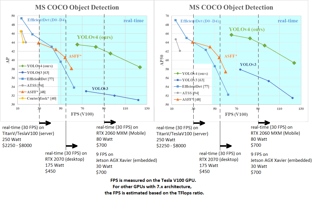
It has a speed of 62 FPS with an mAP of 43.5 percent on the MS COCO dataset.
The y-axis denotes the absolute precision and the x-axis denotes the frame per second (FPS). The blue shaded part of the graph is for real-time detection(webcam, street cameras, etc), and the white is for still detection(pictures). It can be seen that the YOLOv4 does very well in real-time detection, achieving an average precision between 38 and 44, and frames per second between 60 and 120. The YOLOv3 achieves an average precision between 31 and 33 and frames per second between 71 and 120.
This improvement is brought by the inclusion of Bag of Freebies and Bag of Specials.
With this article at OpenGenus, you must have the complete idea of YOLOv4 model architecture.