In this article at OpenGenus, we will start by a general and a mathematical understanding of Kernel Density Estimation and then after exploring some applications of KDE, we, stepwise, implement it in Python. Finally, we talk about the space and time complexity of the python implemenation.

Table of Contents

1. Introduction to KDE
2. Applications of KDE
   a) Data Visualization
   b) Anomaly Detection
3. Step-by-Step Implementation of KDE in Python
   a) Kernel estimation around one point
   b) Estimation around all points in dataset
   c) Sum up estimations to form compound estimations
   d) Get KDE after Normalizing the compound estimations
4. Time and Space Complexity of KDE in Python

Introduction

Kernel Density Estimation is a simple statistical tool to estimate the underlying probability distribution of a given dataset. This means, using KDE one can estimate which data points are most or least likely to be observed when a continuous random variable is measured.

Fundamentally, KDE is achieved by placing a single kernel (usually a bell curve Like a Gaussian ) on each datapoint and then summing these kernels up and finally normalizing the values. The selection of the kernel function plays a crucial role in the shape of the final estimation.
The equation below shows the mathematical formula for calculating the KDE

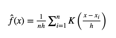
where:
f^(x) represents the estimation function
n is the number of total data points in the dataset
h is the bandwidth of the kernel, sometimes also called the smoothing parameter
xi is a single datapoint in the dataset
K(u) is the kernel function, usually a symmetric and smooth bell curve function

This equation sums up the aforementioned process. The sigma notion shows that for each point the kernel function estimates are summed up and then divided by the number of points for normalization such that the total area under the resulting estimated curve is no more than one!

Applications of Kernel Density Estimation

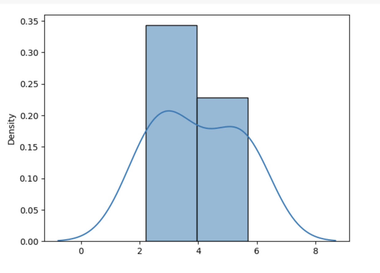
KDE is a beneficial tool for visualizing data distribution in a given continuous dataset. Typtically a histogram is used to understand the distribution of data. However, the problem with this approach is that the histogram uses bins to collect the frequency of points that fall under a bin which means the data points are divided into chunks (bins) and thus the visuals of the distribution are discreet. KDE could be used to present a smooth distribution of the data. The diagram below shows the KDE curve drawn over the histogram.

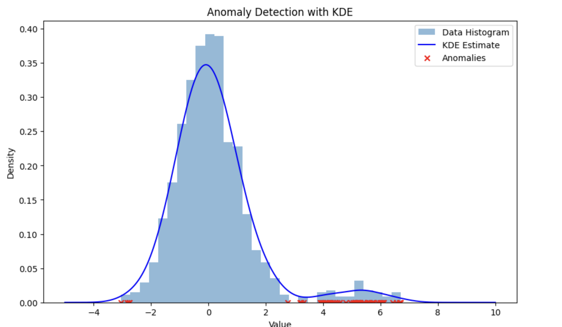
In addition to the visualization application of KDE, it could also be used to detect anomalies such as Credit Card Fraud or anomalies in Sensor Data. Anomaly detection is performed by modeling the probability density of the normal data and then the data points that lie at the edges of the distribution are flagged as potentially anomalous. The diagram below shows how anomalies are detected using KDE. The red points are the potential anomalies.

Implementing KDE in Python

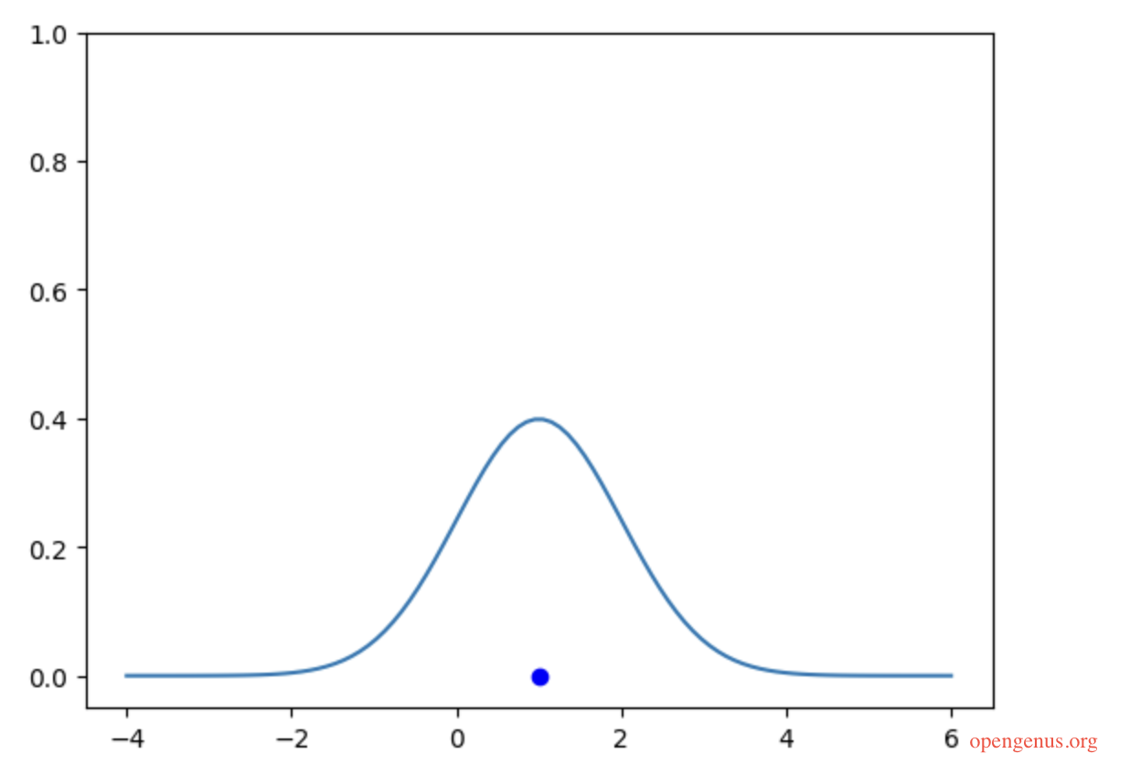
We will start with a simple point on X-axis

point1 = 1
plt.scatter(point1,0, color='b')

Now that we have a point (from our dataset) on the x-axis, let's put a Gaussian Kernel around this point

plt.ylim(-0.05,)
point1 = 1
alpha = 1 #our h value
interval = 5
resolution = 100

x = np.linspace(point1-interval, point1+interval, resolution)
y = np.array([gaussian(pt, point1, alpha) for pt in x])


plt.scatter(point1,0, color='b')
plt.plot(x, y);

We have a point and the kernel distribution applied to that point, let's iterate over all other points in our supposed dataset.

plt.ylim(-0.05,)
datapoints = np.array([2.3, 2.9, 5.1, 6.4])
alpha = 1
interval = 5
resolution = 100

x = np.linspace(datapoints.min()-interval, datapoints.max()+interval, resolution)
for point in datapoints:
  y = np.array([gaussian(pt, point, alpha) for pt in x])
  plt.scatter(point,0, )
  plt.plot(x, y);

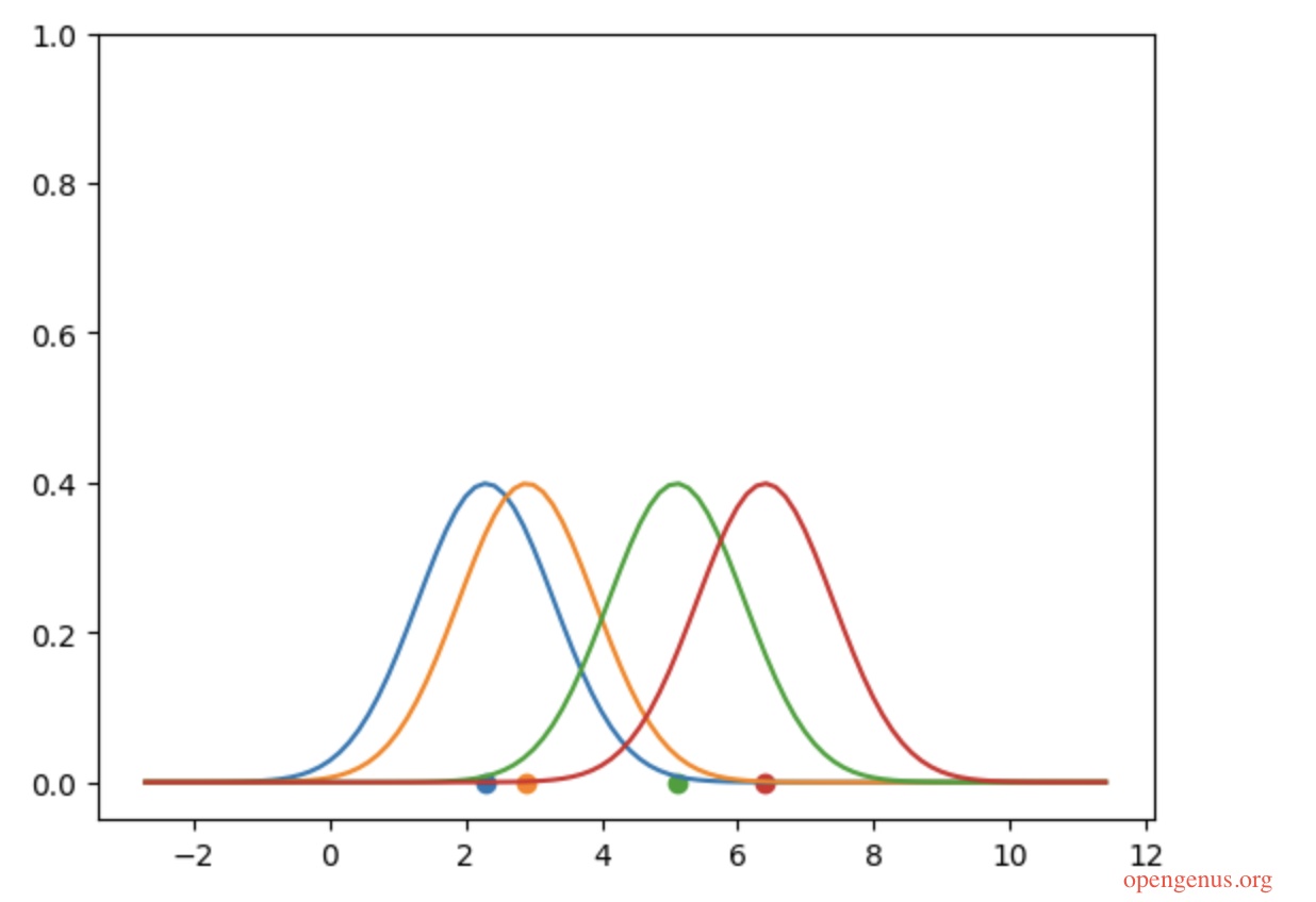
As you can see, there are four points in the datapoints and for each point we have ploted a kernel around it. Summing these kernels up will produce a greater compound effect where points are closer together. The code below shows this.

plt.ylim(-0.05,)
datapoints = np.array([2.3, 2.9, 5.1, 6.4])
alpha = 1
interval = 5
resolution = 100

x = np.linspace(datapoints.min()-interval, datapoints.max()+interval, resolution)
kde_y = np.zeros(resolution)

for point in datapoints:
  y = np.array([gaussian(pt, point, alpha) for pt in x])
  kde_y +=y
  plt.scatter(point,0)
  plt.plot(x, y);
plt.plot(x,kde_y, color='black')

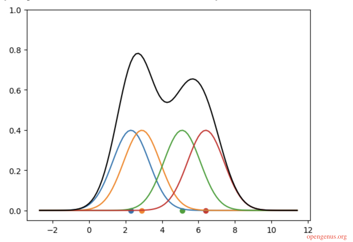
The black curve in the diagram above is supposed to be the KDE of the data points, but there is a slide issue. The sum of the area under a probability distribution curve should always be one. But the area under this curve is far more than that (the area under each kernel is 1, so this curve has 4 kernels under it and a lot more area below the black curve and above the kernels).

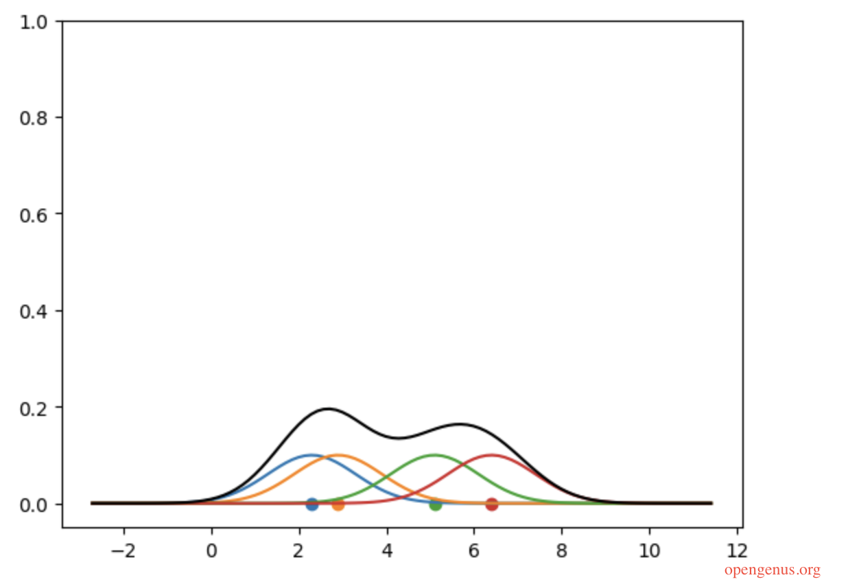
This issue could be dealt with through normalization: simply divide the kde_y values by the number of points!

kde_y /= len(datapoints)
##alternatively divide the y values with len(datapoints)

Time and Space Complexity of KDE in Python

The code above has a main iteration for each point and a nested iteration to estimate density around the each point. This means the time complexity of this algorithm is O(n^2).

The time needed to run this program increases exponentially as the number of points increases in the dataset. In addition, a number of new variables are created in the loop that stores the estimates of density around each point. This means a larger dataset will consume more memory resources. However, it is noteworthy that the resolution of the kernels could be used to limit the size of the list that stores the estimated values of kernels. A smaller resolution might not be as accurate but it will be memory efficient: the challenge is to balance between accuracy and memory efficiency.