
Open-Source Internship opportunity by OpenGenus for programmers. Apply now.
In the ever-evolving landscape of artificial intelligence, where data rules and algorithms reign supreme, one particular challenge stands out: multi-label classification. Imagine a scenario where you need to classify an image not into a single predefined category, but into multiple relevant ones. This intricate task finds its application in diverse domains, from image recognition and medical diagnosis to text categorization and recommendation systems. Delving into the intricacies of multi-label classification promises a fascinating journey that combines mathematical prowess with creative problem-solving.
Table of Contents
- Unveiling Multi-Label Classification
- Tackling the Complexity
- Accuracy and Performance in Multi-Label Classification
- Illuminating the Differences
- Mathematical Insights: Hamming Loss
- Deep Learning Models for Multi-Label Classification
- Enhancing Multi-Label Classification with Neural Networks
- Visualizing the Concepts
- Ethical Considerations: The Path of Responsible AI
- Conclusion: Your Journey Awaits
1. Unveiling Multi-Label Classification
At its core, multi-label classification involves assigning multiple labels or categories to a given data point. Unlike traditional single-label classification, where an input belongs exclusively to one class, multi-label classification reflects the complex reality that real-world entities often belong to more than one category. Imagine an image of a furry friend: it could be labeled as both "dog" and "adorable," capturing various aspects simultaneously.
Mathematically, think of a dataset as a matrix where rows represent data points, and columns correspond to possible labels. Each entry in the matrix indicates the presence (1) or absence (0) of a label for a particular data point. The goal of a multi-label classification algorithm is to predict these binary label vectors accurately.
2. Tackling the Complexity
Multi-label classification's complexity stems from several aspects, each posing a unique challenge that algorithms must navigate to provide meaningful and accurate predictions.
2.A. Variable Number of Labels per Instance
Unlike single-label classification, where an instance belongs to a single category, multi-label classification embraces the reality that instances can possess multiple attributes or characteristics simultaneously. For instance, an image can be labeled as both "sunny" and "beach," highlighting the inherent complexity in capturing diverse features. Algorithms need to account for this variability when making predictions, demanding a flexible approach that accommodates these overlapping attributes.
2.B. Label Correlations: Unveiling Hidden Relationships
In the real world, labels rarely exist in isolation; they often hold intricate relationships. Imagine an image of a sun-kissed beach; it might be associated with labels like "ocean," "sand," and "sun." Understanding and capturing these label dependencies is crucial for accurate predictions. Techniques like label graph models depict labels as nodes and correlations as edges, enabling algorithms to unravel these connections effectively. By leveraging these relationships, models can enhance their predictive power by considering the contextual associations between labels.
2.C. Potential Label Imbalance: Balancing Act
Multi-label datasets might exhibit label imbalance, where certain labels are more prevalent than others. This can skew the learning process, as algorithms might become biased towards predicting the dominant labels while neglecting the less frequent ones. Balancing this disparity requires careful preprocessing techniques, such as oversampling or undersampling, to ensure that the model doesn't prioritize certain labels at the expense of others. Striking this balance is vital for achieving a well-rounded and accurate classifier.
2.D. Evaluation Metrics: Gauging Performance Holistically
Evaluating the performance of multi-label classifiers introduces new challenges due to the intricate nature of label assignments. Traditional accuracy, which works well in single-label classification, falls short here due to the possibility of partial correctness in predictions. In response, specialized metrics step in to provide a holistic view of classifier performance.
-
Hamming Loss: This metric quantifies the proportion of incorrectly predicted labels across all instances. It provides insights into how well the classifier is capturing the labels' complexities.
-
Subset Accuracy: Unlike traditional accuracy, subset accuracy considers an instance as correctly classified only if all its labels are predicted correctly. This metric accounts for the inherent difficulty of predicting multiple labels accurately.
-
F1-Score: Adapted for multi-label scenarios, the F1-Score combines precision and recall to evaluate classifier performance. It considers false positives, false negatives, and true positives for each label, providing a balanced assessment.
3. Accuracy and Performance in Multi-Label Classification
In the realm of multi-label classification, achieving accuracy is an intricate pursuit that involves navigating a spectrum of challenges to predict labels that effectively capture the nuanced attributes of real-world instances. This journey combines mathematical prowess with creative problem-solving, ultimately resulting in robust classifier performance. Here, we delve into the strategies and algorithms that contribute to accurate multi-label classification.
3.A. Striving for Accurate Multi-Label Classification
Accurate multi-label classification involves accurately predicting multiple relevant labels for each instance in a dataset. While traditional accuracy is a common metric for single-label classification tasks, it is not directly applicable to multi-label scenarios due to the complex nature of label assignments.
Top-1 Accuracy and Multi-Label Classification
In multi-label classification, the notion of "top-1 accuracy" does not fully capture the model's performance. Traditional top-1 accuracy measures whether the highest predicted label matches the true label for a single-label classification task. However, in multi-label classification, instances can have multiple correct labels, and a single top-1 prediction might not adequately reflect the model's ability to capture all relevant labels.
Achieving accurate multi-label classification involves navigating various challenges to predict labels that capture the nuanced attributes of real-world instances. Key strategies include:
-
Understanding Label Interplay: Recognizing label dependencies and correlations is crucial. Techniques like label graph models can unravel hidden relationships and improve prediction accuracy.
-
Mitigating Label Imbalance: Preprocessing techniques like oversampling or undersampling address label imbalance, ensuring that the model doesn't prioritize dominant labels over less frequent ones.
-
Choosing Appropriate Metrics: Traditional accuracy falls short in multi-label scenarios. Metrics like Hamming Loss, Subset Accuracy, and F1-Score provide a comprehensive view of classifier performance.
3.B. Algorithms at Play: Navigating Complexity
Several algorithms are designed to handle the complexity of multi-label classification:
-
Binary Relevance: Binary Relevance is a straightforward approach that treats each label as an independent binary classification problem. Essentially, you create a separate binary classifier for each label. When predicting labels for an instance, each binary classifier operates independently to decide whether the corresponding label should be assigned to the instance. This approach is simple and allows existing single-label classification algorithms to be used for each label, but it might not consider label correlations.
-
Label Powerset: The Label Powerset approach transforms the multi-label classification problem into a multi-class classification problem. Each unique combination of labels in the dataset is treated as a separate class. The model then predicts the most appropriate combination of labels for an instance. While this approach captures label dependencies, it can suffer from the curse of dimensionality when dealing with a large number of labels.
-
Classifier Chains: Classifier Chains extends the Label Powerset approach by considering label order and correlations. The idea is to train a sequence of binary classifiers, where each classifier takes into account the predictions of the previous classifiers in the sequence. This method accounts for label dependencies and captures their order, which can be important in cases where labels have a natural sequence or hierarchy.
These algorithms attempt to address the intricacies of multi-label classification by adapting existing single-label classification methods or introducing new strategies to handle label dependencies and correlations. Choosing the right algorithm depends on the characteristics of the dataset and the problem you're trying to solve.
4. Illuminating the Differences
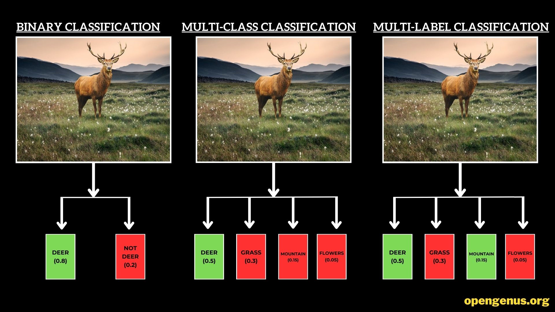
Illustration showcasing the differences between binary classification, multi-class classification, and multi-label classification.
Binary Classification: Simple Yet Profound
Binary classification, often regarded as the foundation of classification tasks, operates in a straightforward manner: instances are categorized into one of two classes. This binary decision-making process has broad applications, from spam detection in emails to medical diagnosis. In this scenario, the algorithm discerns whether an instance belongs to the positive class (1) or the negative class (0), offering a clear-cut answer.
Multi-Class Classification: Beyond Black and White
Multi-class classification takes a step beyond binary decision-making, accommodating instances that can belong to one of several classes. Picture a scenario where images of animals need to be sorted into categories like "deer," "grass," and "mountains." The image is assigned a single label representing its most fitting class, in this case it is Deer. This diverse classification type enables systems to handle a wide array of possibilities and is pivotal in applications like language translation or character recognition.
Multi-Label Classification: Navigating Complexity
In the realm of multi-label classification, instances are not confined to a single label but can be associated with multiple labels simultaneously. This dynamic approach acknowledges the multifaceted nature of real-world entities. For instance, consider an image depicting a serene landscape featuring a majestic deer grazing on grass, surrounded by towering mountains. This image defies binary or single-class assignment—it's a symphony of attributes that demand a multi-label classification. This complexity is encountered in various domains, such as image tagging, where a single image might carry multiple labels like "deer," "grass," and "mountains."
The distinction between these classification types lies in the granularity of decision-making. While binary classification simplifies choices into two categories, multi-class classification widens the spectrum, and multi-label classification navigates the intricate terrain of multiple attributes per instance. As we delve into these classification realms, the algorithms and techniques employed become increasingly sophisticated, reflecting the nuances of the real world they aim to replicate.
5. Mathematical Insights: Hamming Loss
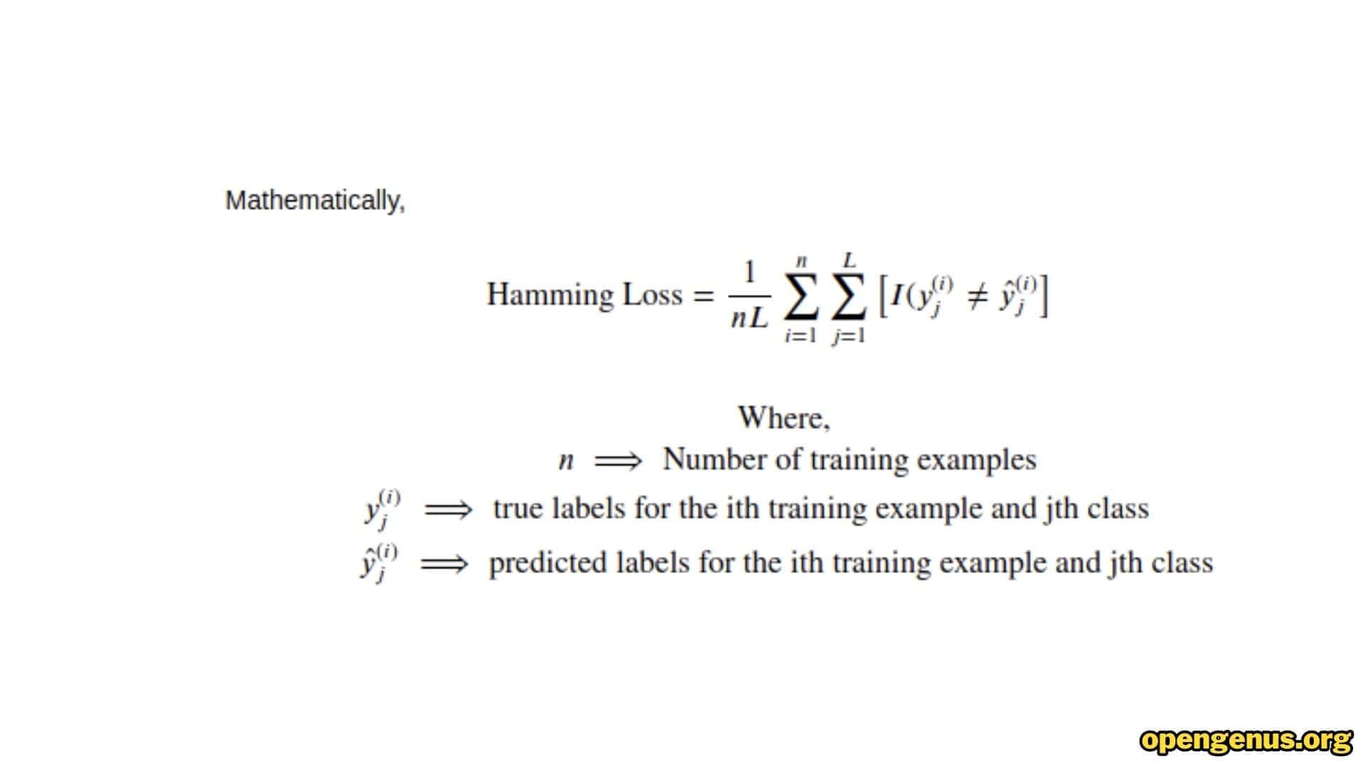
Mathematical representation of Hamming Loss.
In multi-label classification, the Hamming Loss metric plays a pivotal role in assessing the accuracy of label predictions. This mathematical concept provides valuable insights into the performance of a classifier when dealing with the intricacies of multi-label assignments.
The Hamming Loss formula is represented as follows:
Hamming Loss = (1 / N) × ∑i=1N H(yi, yhat,i)
Where:
- N is the number of instances,
- yi represents the true label vector for the i-th instance,
- yhat,i represents the predicted label vector for the i-th instance, and
- H(yi, yhat,i) calculates the Hamming loss between the true and predicted label vectors.
The Hamming Loss formula then aggregates these individual Hamming losses for all instances and computes the average. The resulting value lies between 0 and 1, where a lower value indicates better performance. A Hamming Loss value of 0 indicates perfect predictions, while a value of 1 means that all labels are predicted incorrectly for all instances.
For example
Imagine you have a dataset of images, and each image can be associated with multiple labels. For instance, an image of a sunny beach can be labeled with "ocean," "sand," and "sun." Let's say you have a total of 5 images and 3 possible labels: "ocean," "sand," and "sun."
Now, let's assume you've trained a multi-label classifier on this dataset, and it's making predictions for each label on each image. Here's a hypothetical scenario of predicted labels for each image:
| Image | Predicted Labels | True Labels |
|---|---|---|
| 1 | ocean, sun | ocean, sand |
| 2 | sand | sand |
| 3 | ocean, sun, sand | ocean, sun, sand |
| 4 | sun | sun |
| 5 | ocean, sand, sun | sand, sun |
In this scenario, the classifier's predictions are compared to the true labels for each image. The Hamming Loss is then calculated based on these comparisons.
Calculating Hamming Loss
For each instance (image), the Hamming Loss is calculated by counting the number of labels that are predicted incorrectly and dividing it by the total number of labels. The Hamming Loss is then averaged across all instances in the dataset.
In the example above, the Hamming Loss for each image is as follows:
- Hamming Loss for Image 1: 1/3 (1 label predicted incorrectly out of 3)
- Hamming Loss for Image 2: 0/3 (0 labels predicted incorrectly out of 3)
- Hamming Loss for Image 3: 0/3 (0 labels predicted incorrectly out of 3)
- Hamming Loss for Image 4: 0/3 (0 labels predicted incorrectly out of 3)
- Hamming Loss for Image 5: 1/3 (1 label predicted incorrectly out of 3)
Average Hamming Loss = (1/3 + 0/3 + 0/3 + 0/3 + 1/3) / 5 = 2/15 ≈ 0.133
Output Representation
The output of Hamming Loss is a single scalar value that ranges between 0 and 1. In this case, the Hamming Loss of approximately 0.133 indicates that, on average, about 13.3% of the labels are predicted incorrectly across all instances in the dataset. Lower values of Hamming Loss indicate better performance, while a value of 0 would mean that all labels are predicted perfectly.
In multi-label classification scenarios, the Hamming Loss provides valuable insights into how well the classifier is capturing the complexities of label assignments across multiple instances.
Another example
let's say you have a multi-label classifier for image recognition with 1000 possible labels. The output layer might look like this:
Label 1: 0.85
Label 2: 0.23
Label 3: 0.60
...
Label 1000: 0.05
In this output representation, each probability value represents the confidence of the model in predicting the presence of a particular label. For instance, a probability of 0.85 for "Label 1" indicates that the model believes the image contains the object associated with that label with a high level of confidence.
In summary, the output of Hamming Loss is a single value that quantifies how well a multi-label classification model predicts labels across multiple instances. It serves as a comprehensive evaluation metric that considers the complex nature of multi-label assignments.
6. Deep Learning Models for Multi-Label Classification
Several deep learning models have proven effective for multi-label classification tasks, leveraging their ability to process complex data and capture intricate label relationships:
-
Convolutional Neural Networks (CNNs): CNNs excel in image-based multi-label classification tasks by extracting hierarchical features from images. They can simultaneously identify multiple objects within an image, making them suitable for tasks like image tagging and recognition.
-
Recurrent Neural Networks (RNNs): RNNs are well-suited for sequential data such as text and time-series information. Their temporal understanding enables them to capture label dependencies in tasks like text categorization or sentiment analysis.
-
Transformer Models: Transformers, with their attention mechanisms, excel in processing sequences and capturing long-range dependencies. They are highly effective for tasks involving natural language processing, text classification, and document categorization.
-
Graph Neural Networks (GNNs): GNNs are valuable for multi-label tasks involving data with inherent graph structures. They can model label correlations within graphs, making them suitable for recommendation systems, social network analysis, and bioinformatics.
These deep learning models empower multi-label classification by learning intricate patterns, hierarchies, and label dependencies present in the data. Their versatility makes them valuable tools for addressing the complexities of multi-label assignments across various domains.
7. Enhancing Multi-Label Classification with Neural Networks
Neural networks, particularly Convolutional Neural Networks (CNNs), have proven to be effective tools for multi-label image classification tasks. Common CNN architectures, like MobileNetV1, that are originally designed for single-label image recognition can be adapted and extended to handle multi-label classification scenarios. Here's how:
Adapting CNN Models for Multi-Label Classification
-
MobileNetV1 and Multi-Label Classification
MobileNetV1 is a lightweight CNN architecture designed for image classification tasks. In a multi-label classification scenario, MobileNetV1 can be adapted in the following ways:
-
Output Layer: In single-label classification, the output layer typically has neurons corresponding to the number of classes. In multi-label classification, the output layer would have neurons corresponding to the number of possible labels. Each neuron's activation function can be a sigmoid function, allowing each neuron to independently predict the presence or absence of a label.
-
Loss Function: The loss function used for training would need to change. Binary Cross-Entropy Loss is commonly used for multi-label classification, as it's suitable for modeling independent binary label predictions.
-
Activation Function: Since multi-label classification involves independent predictions for each label, the activation function in the output layer should be a sigmoid function instead of softmax. This allows for multiple labels to be predicted simultaneously.
-
Other CNN Models for Multi-Label Classification
-
ResNet-50 for Multi-Label Classification
ResNet-50 is a deep CNN architecture known for its deep layer structure. For multi-label classification:
-
Output Layer: Similar to MobileNetV1, the output layer would have multiple neurons corresponding to the number of labels, each with a sigmoid activation function.
-
Fine-Tuning: Pre-trained ResNet-50 models can be fine-tuned on multi-label datasets to adapt the learned features to the task.
-
-
InceptionV3 for Multi-Label Classification
InceptionV3 is another CNN architecture known for its use of multiple parallel convolutional paths. To adapt InceptionV3 for multi-label classification:
-
Output Layer: The output layer structure remains the same, with multiple sigmoid-activated neurons.
-
Feature Extraction: The unique feature extraction capabilities of InceptionV3 can help capture complex patterns within multi-label images.
-
-
VGG16 for Multi-Label Classification
VGG16 is a CNN architecture characterized by its deep layers with small convolutional filters. To use VGG16 for multi-label classification:
-
Output Layer: As before, the output layer is modified to accommodate multiple labels with sigmoid activation.
-
Transfer Learning: Pre-trained VGG16 models can be fine-tuned or used for feature extraction on multi-label datasets.
-
These adaptations demonstrate that common CNN models can be effectively repurposed for multi-label classification by adjusting the architecture of the output layer, loss functions, and activation functions. It's important to note that while the core architecture remains similar, these modifications enable the models to handle the complexities of multi-label assignments and make independent label predictions.
Architectural Changes Illustrated
Adapting MobileNetV1 for Multi-Label Classification:
Original MobileNetV1 Architecture:
Input → Convolutional Layers → Fully Connected Output Layer (softmax activation)
Modified MobileNetV1 Architecture for Multi-Label Classification:
Input → Convolutional Layers → Fully Connected Layer (sigmoid activation)
In the modified architecture, the softmax activation in the output layer is replaced with sigmoid activation. Additionally, the number of output neurons in the fully connected layer corresponds to the number of labels in the dataset. These architectural changes enable MobileNetV1 to predict the presence of multiple labels for each image, aligning with the complexities of multi-label classification tasks.
Adapting ResNet-50, InceptionV3, and VGG16 for Multi-Label Classification:
The architectural changes for adapting ResNet-50, InceptionV3, and VGG16 for multi-label classification follow a similar pattern:
-
Output Layer Modification: The output layer structure is modified to have multiple neurons, each representing a label, with a sigmoid activation function.
-
Fine-Tuning or Transfer Learning: Pre-trained models can be fine-tuned on multi-label datasets, or used for feature extraction. This allows the models to learn relevant features specific to the multi-label task.
These adaptations empower these well-known CNN architectures to effectively predict multiple labels, making them suitable for the nuanced challenges of multi-label classification tasks. By embracing these changes, these models can handle instances where an image can belong to more than one category simultaneously.
8. Visualizing the Concepts
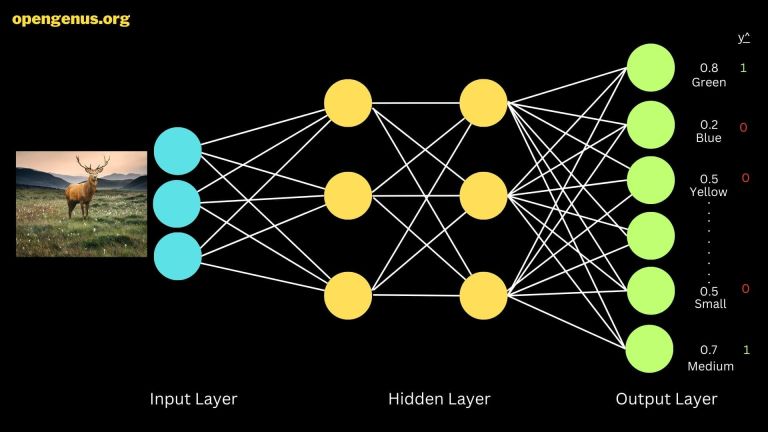
Visualization of a neural network architecture for multi-label classification.
This visual encapsulates multi-label classification within a neural network. The image unfolds a process where an input layer receives a deer image. Hidden layers process this input, extracting features. The output layer showcases predictions.
Labels like "green," "blue," "small," and "medium" are represented with intensities, indicating the network's confidence. High intensity, like 0.8, implies certainty, while 0.6 suggests moderate confidence.
Outcome is shown through y hat values—binary indicators. A y hat of 1 signifies affirmation of a label, e.g., "green" or "medium," while other labels get 0, implying their absence.
This image showcases neural networks' ability to decode complex attributes and predict multiple features simultaneously.
9. Ethical Considerations: The Path of Responsible AI
As AI technology evolves, the ethical landscape of multi-label classification becomes increasingly critical. Responsible use of AI's predictive capabilities is essential to avoid unintended consequences and biases.
Ensuring Unbiased Predictions: Multi-label classifiers must guard against perpetuating biases present in training data. Historical disparities and societal inequalities can lead to skewed predictions, unfairly affecting certain groups. Rigorous data curation, bias detection mechanisms, and fairness-aware training are essential to address these issues and ensure equitable outcomes.
Addressing Privacy and Fairness Concerns: Multi-label classification may inadvertently reveal sensitive individual information. Ethical concerns arise when predictions involve personal attributes like health conditions or political affiliations. Robust privacy-preserving techniques, such as differential privacy and secure multi-party computation, are crucial to safeguard sensitive information while deriving insights from multi-label data.
Balancing AI Advancement and Ethical Responsibility: The advancement of multi-label classification must align with ethical principles. Achieving a harmonious balance between innovation and responsible deployment requires collaboration among AI researchers, developers, policymakers, and society. Ethical guidelines, transparency, and ongoing audits are essential to ensure that multi-label classification technologies empower rather than harm individuals and communities.
In the journey of mastering multi-label classification, it's crucial to consider not only technical prowess but also ethical dimensions. By integrating responsible practices into the development and deployment of multi-label classifiers, we can pave a path toward AI systems that are both effective and ethical, benefiting individuals and society as a whole.
10. Conclusion: Your Journey Awaits
Multi-label classification embodies the complex beauty of AI challenges. Its applications span diverse fields, from healthcare to entertainment. To master this realm, cultivate technical prowess, nurture creative thinking, and stoke the fires of curiosity. The OpenGenus internship propels you into this captivating domain, equipping aspiring AI enthusiasts to not only understand multi-label classification but also drive its evolution. Embark on this journey, and let the dynamic world of multi-label classification become your canvas of innovation.