Backtracking is one of the many algorithmic techniques that can be used to solve various problems. In this article, we will exploring the idea of backtracking with the help of recursion (Recursive Backtracking) along with examples as well.

Table of content:

1. What is Recursion?
2. Visualization of Recursion & Memory usage
3. What is Backtracking? (+ Recursive Backtracking)
4. Visualization of Backtracking along with an example
5. Advantages of Backtracking

We will get started now.

1. What is Recursion?

In order for us to understand what backtracking is, we need to be very familiar with the concept of recursion.

In a programming setting, a method or function that calls itself is a recursive function. Generally, a recursive method solves a problem by calling a copy of itself to work on a smaller problem. This is known as the recursion step. This particular recursion step can result in many more such recursive calls.

You might be wondering though, how does the method know that it is time to stop the recursive calls, i.e., stop calling itself?

Well, it is very important that the recursive calls stop at some point, and it is the programmer's responsibility to make sure that happens. All recursive methods and functions have a base case and the recursive calls stop because of them. The sequence of smaller problems must eventually converge on the base case.
Generally speaking, a recursive function usually has the following structure:

define recursiveFunction(data) as:
    if (check for base condition):
        return some value
    else if (check for some other base condition):
        return some value
    else:
        //Perform some computations here
        recursiveFunction(data)

As an example, to calculate the factorial of any number, we would have the following recursive function:

def factorial(n):
    if n==0: return 1
    return n * factorial(n-1)
    
print(factorial(6))

The base case for the above program is if the value of n becomes 0, simply return 1.
It generates the following output:

720

2. Visualization of Recursion & Memory usage

Each time a new recursive call is made, a new copy of that method (its variables) is generated and stored in memory. Once that recursive call is complete or terminated, the copy of that method is also removed from the memory.

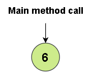
To better understand recursion, let us visualize the factorial program that we wrote in the previous section.

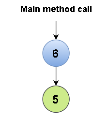
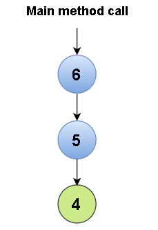
Let us denote the function or method calls by a node.

• First we call the main factorial method by passing 6 as the parameter.
  
• Inside the function, another recursive call is made as follows:
  factorial(n-1)
  Since n = 6, factorial(6-1) = factorial(5)
  This time 5 will be passed as our parameter.
  
• Another recursive call will be made as follows:
  factorial(n-1)
  Since n = 5 (for the copy that has been stored for this recursive call, remember how the memory storage works for recursive functions), factorial(5-1) = factorial(4)
  This time 4 will be passed as our parameter.
  
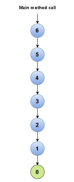
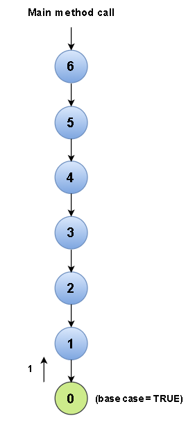
• The same methodology will be followed until the base case for this recursive function becomes true, i.e., the value of n becomes 0.
  The structure will now look something like this.
  
• Since the value of n has now become 0 (in our latest recursive call), the base case has become true and so we will simply return the value of 1 to the original call.
  
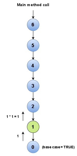
• Now, coming back to our previous call (where n was equal to 1), we have to return the following to the original call:
  n * factorial(n-1)
  Since n = 1 and factorial(n-1) returned the value of 1, we shall simply return 1 * 1 = 1 to the original call.
  
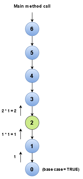
• Now, coming back to our previous call (where n was equal to 2), we have to return the following to the original call:
  n * factorial(n-1)
  Since n = 2 and factorial(n-1) returned the value of 1, we shall simply return 2 * 1 = 2 to the original call.
  
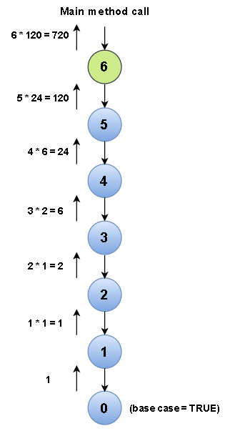
• Once again, the same methodology will be followed until we reach the main function call (from the driver program), where the value of 6 * 120 = 720 will be returned.
  
• The function finally returns the value of 720, and hence we now have our final answer (6! = 720).

3. What is Backtracking?

Backtracking is a general algorithm in which a systematic search for a solution to a particular problem among all the available options is performed.

In backtracking, we usually we start with one possible option out of many available options and then sequentially try to solve the problem. If we are able to solve the problem with the selected choice/move, then we can simply return the answer or else we can backtrack and select some other option and then try solving the problem. This way, we can either :

(a) Find the solution to the problem, in which case we can simply return the answer, or
(b) Exhaust/Run out of all the options without finding a solution, in which case we can claim that there is no solution to the given problem.

By now, you should have guessed that backtracking is simply a form of recursion. In backtracking, we have a number of options available to us and we must choose one of those options. After making a selection, we get a new set of options and then these steps are repeated until we find a solution to the problem. If a solution is not found with a particular set of options/moves, then we can backtrack and try out a different set of options or moves. This process is repeated until we reach a final state.

4. Visualization of Backtracking along with an example

Now that we understand as to what backtracking is, let us try and solve a problem with the help of backtracking so that we can further familiarize ourselves with this technique.

Pathfinding Problem: You are given a 2D matrix with n rows and m columns. This matrix only consists of 0 and 1 as its elements, where 0 represents a wall and 1 represents a path. Given a starting position (s1, s2), check if it is possible to reach the given ending position (e1, e2). If it is possible to reach the ending position, return the path that can be taken in order to reach it from the starting position. Note that you can only move in the forward and downward direction.
Suppose we have a matrix:

[
[1, 1, 1, 1],
[1, 0, 1, 1],
[0, 1, 1, 1],
[0, 1, 0, 1]
]

Given, starting position = (s1, s2) = (0, 0)
ending position = (e1, e2) = (3, 3)

It is clear that we can reach the ending position through multiple paths. We can simply display one of these paths as our final answer. For example, the following output would suffice:
Path taken = (0, 0) => (0, 1) => (0, 2) => (0, 3) => (1, 3) => (2, 3) => (3,3)

Intuitive algorithm:
The following steps are to be repeated (since they are recursive in nature) until a final state has been reached:

1. If the exit position has been reached, simply return the co-ordinates of our current position (exit position itself).
2. Else, move in the downward direction and check if it leads to the solution.
3. If the downward direction seems unfeasible, move in the forward direction.
4. If both seem feasible, choose either one of them and move ahead with the rest of the problem.
5. If a dead-end is reached, simply backtrack and explore other options.

Backtracking solution:

def pathFinder(matrix, startPos, endPos):
    if startPos == endPos:
        return [startPos]
    x, y = startPos[0], startPos[1]
    if x + 1 <= endPos[0] and matrix[x+1][y] == 1:
        path1 = pathFinder(matrix, (x+1, y), endPos)
        if path1:
            return [(x, y)] + path1
    if y + 1 <= endPos[1] and matrix[x][y+1] == 1:
        path2 = pathFinder(matrix, (x, y+1), endPos)
        if path2:
            return [(x, y)] + path2

if __name__ == "__main__":
    matrix = [
             [1, 1, 1, 1],
             [1, 0, 1, 1],
             [0, 1, 1, 1],
             [0, 1, 0, 1]
             ]
    startPos, endPos = (0, 0), (3, 3)
    print(*pathFinder(matrix, startPos, endPos), sep=" ==> ")

The above program generates the following output:

(0, 0) ==> (0, 1) ==> (0, 2) ==> (1, 2) ==> (2, 2) ==> (2, 3) ==> (3, 3)

The complete visualization of the working of this program has been described below.
Each node represents a separate function call with a different set of parameters and the red text and symbols are used when something is returned by a particular call or function.

Time complexity: If the input matrix has r rows and c columns and a constant amount of work K is being done in each call, then time complexity of our algorithm should be O(r * c) + K. We can ignore the constant.
Hence, the overall time complexity should be O(r * c).

Space complexity: Since our algorithm has a recursive nature, its overall space complexity is also going to be O(r * c).

5. Advantages of Backtracking

1. Backtracking is an effective way to solve problems with some given constraints.
2. Backtracking is always going to return a solution to the problem, else we can claim that a solution doesn't exist to the problem.
3. It can be easily incorporated into other algorithms.
4. Various states (parameters, local variables, etc.) of different calls are saved into a stack, so that they can be re-used somewhere down the line.
5. Backtracking algorithms are used in various fields such as artificial intelligence, electrical engineering, robotics,etc.

With this article at OpenGenus, you must have the complete idea of Recursive Backtracking.