In this article, I introduce calibration in Machine Learning and Deep Learning, an useful concept that not many people know.

Table of contents:

I. What is calibration?
II. Why do we need calibration?
III. When do we use calibration?
IV. How do we use calibration?
1. Assessing calibration
2. Calibration methods
V. Conclusion

I. What is calibration?

Calibration is defined as a way of making a pre-trained model predict probability of outputs more accurately and increasing its confidence about outputs.

Come to the next question :

II. Why do we need calibration?

Many practitioners often errorneously misunderstand probability obtained from models as their confidence.Actually, even with a high probability prediction of an event,models still don't have high confidence about it.

For instance, suppose that you have trained a neuron network to classify images of cats and dogs.You use this model on test set to predict probability of some samples.
Divide probability into 5 bins with step = 0.2.Say that if you predict an image of being cat with probability 0.1, put it in bin [0,0.2].Repeat with other samples and we get the result here :

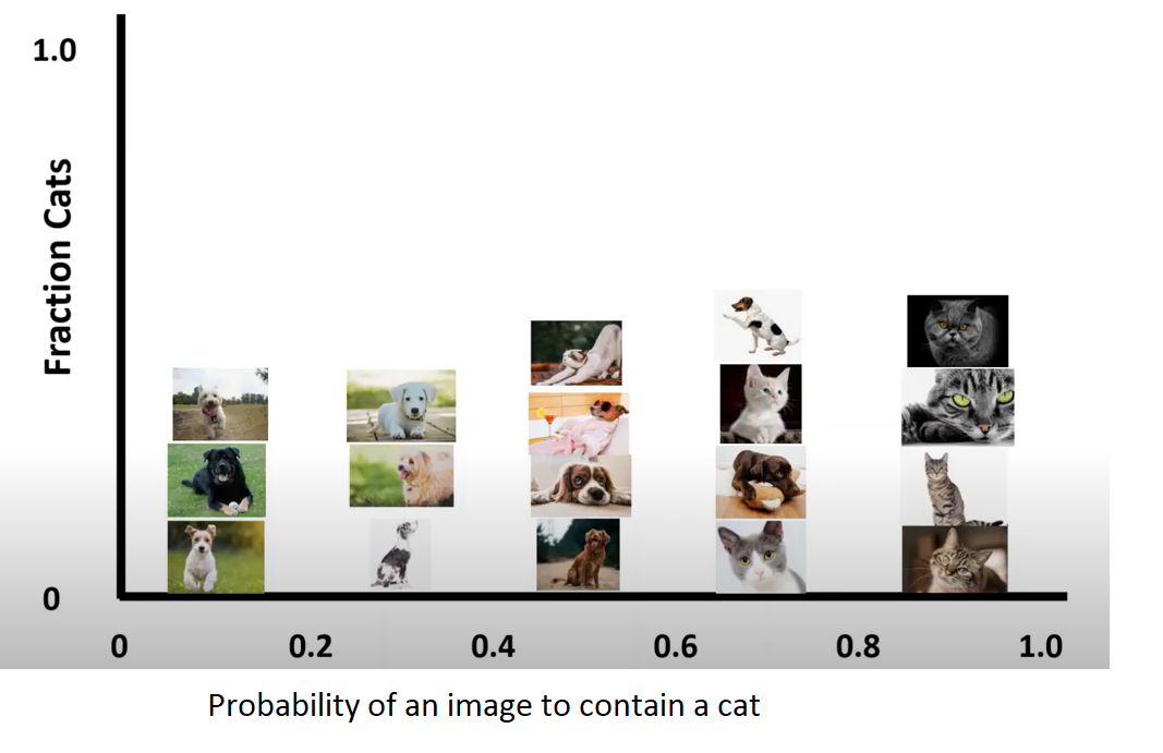
Let's analyze to understand more.In the picture above,your model predicted 4 images of being cat with probability lying in bin [0.4,0.6].Therefore, we might expect the number of cat images account for 50% of total images.But if you look carefully, there is only one image of cat in total 4 images,so fraction of cat images is only 25%!Marking this point with orange "X" , and connecting everything:

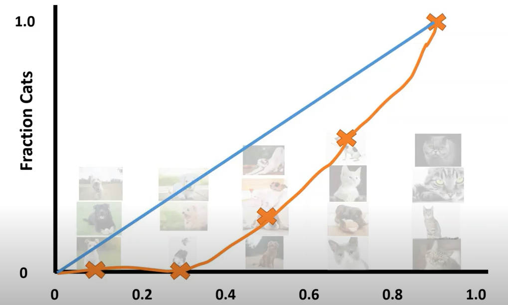
Note that the blue line is perfectly calibrated predictive line of model that we expect , whereas the orange one is the true predictive line of our model. There is a big gap between them, and we can say that our model is not well-calibrated.This plot is called 'Reliability diagram' which we will discuss below.
Hope that now you got the answer for the question above.

III. When do we use calibration?

You can utilize this technique whenever you want to increase confidence of you models,especially if you realize that your model was not well-calibrated.
Anyway, it is applied commonly in some specific cases that require very high accuracy like medical treatment,controlling process in nuclear power plant,etc...Take an example,you are trying to build a machine learning model to explore and predict the effect of a new drug, you should use this technique to make your model better unless you want to be thrown in jail because your drug caused the death of many patients.

IV. How do we use calibration?

Before we calibrate some network, we need to know whether our model was calibrated.Only by doing this, we could know if our model really need to be calibrated or the calibration method helps our model better.
Inspite of the large number of metrics, I only two common ones to assess calibration.

1. Assessing calibration.

1.1.Brier Score.

Brier score is actually a fancy name of mean square error of true label and predicted probability.

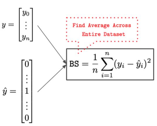
Although Brier score is a good metric to measure model's prediction, it doesn't say anything about probabilities associated with infrequent events.Thus, we should utilize other metrics in addition to BS to get more useful insights.
In practice, for convenience,sklearn provides a good function to measure use this metrics:

from sklearn.metrics import brier_score_loss
brier_score_loss(y_test_1, rf1_preds_test_uncalib) # y_test_1 is the true label of test set,rf1_preds_test_uncalib is predicted probability of random forest model

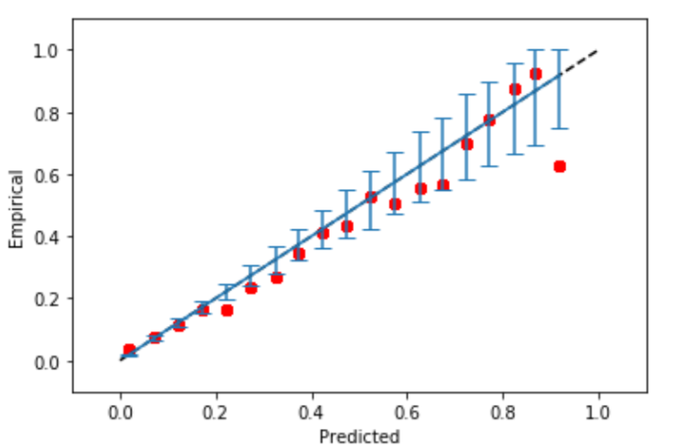
1.2.Reliability diagram.

This is a visual way to check calibration of models and we have seen it in the picture above.It is composed of two components:

• X_axis depicts predicted probabilities(i.e. average confidence) in the interval [0,1]
• y_axis expresses empirical probabilities or perfect calibration.

To plot reliability diagram, folowwing those steps:

• Divide the interval [0,1] into smaller subset,e.g.[0,0.2],[0.2,0.4],...[0.8,1.0]
• Put instances in each bin based on their predicted probability.
• Find the empirical(expected)probability of each sample(e.g. if there are 9 images of cats out of 20 total images, we get 9/20=0.45).
• Connect all the dots,plot the predicted probability line and perfect calibration line.
• When the dots are (significantly) above the line y=x, the model is under predicting the true probability, if below the line, model is over-predicting the true probability.
  To use this diagram, we need to import module ml_insights

import ml_insights as mli
# This is the default plot
rd = mli.plot_reliability_diagram(y_test_1, rf1_preds_test_uncalib)

And we derive the plot:

2. Calibration methods

In this part, I introduce 2 common methods which belong to two different categories.

2.1.Platt scaling

Platt scaling is a parametric approach which uses the the non-probabilistic predictions of our model as input of logistic regression.
Logistic regression uses sigmoid function to predict the true probability of samples:

P_i = 1 / [1 + exp^{(A fi + B)}]

where fi = f(x) that is output of the model at a given data point x.

Note that A and B are parameters of logistic regression and our goal is to learn them.F(x) is the non-probabilistic output of our model as we discussed.
To get the best params, use gradient descent.

Some pros and cons of Platt scaling:

• Very restrictive set of possible function
• Need very little data

Try to write code to see what happens:

# Fit Platt scaling (logistic calibration)
lr = LogisticRegression(C=99999999999, solver='lbfgs')
lr.fit(calibset_preds_uncalib_1.reshape(-1,1), y_calib_1)

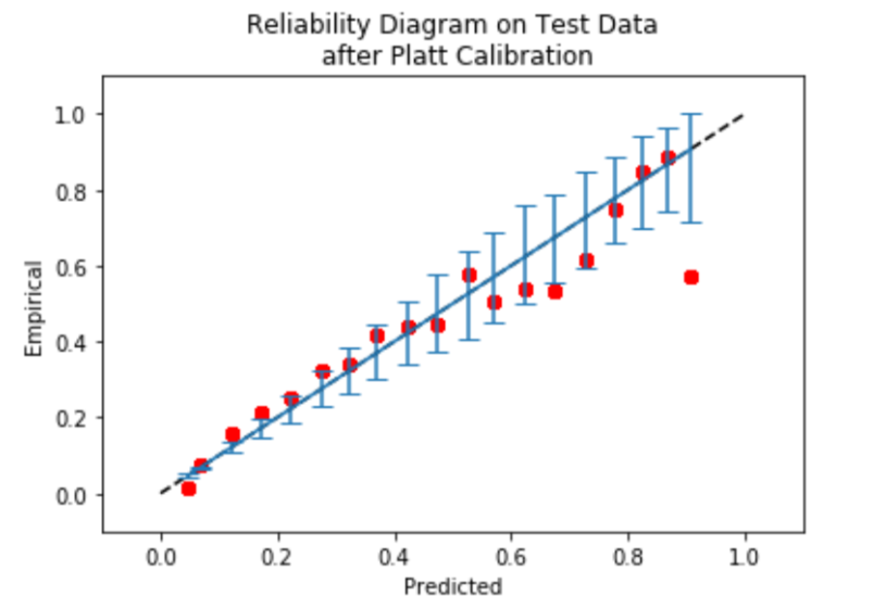
After calibration, we can plot reliability diagram to know if our model was well-calibrated:

mli.plot_reliability_diagram(y_test_1, testset_platt_probs)
plt.title('Reliability Diagram on Test Data\n after Platt Calibration')

2.2.Isotonic regression

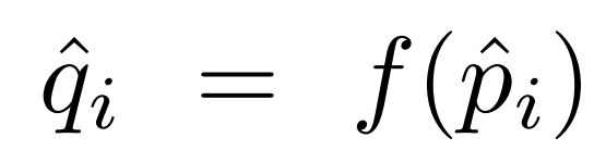
Isotonic is arguably the most common non-parametric approach, tries to learn a piecewise constant,non-decreasing function to transform uncalibrated outputs.If our model predicts output with p^i value then the relationship between p^i and the distribution that we expect can expressd by this fomular:

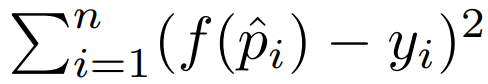
where f is the isotonic function. Our goal is to minimize the square loss:

Some advantages and disadvantages of this method:

• Tends to better than Platt scaling with enough data
• Tends to be overfit

Let's try to apply this algorithm.

from sklearn.isotonic import IsotonicRegression
iso = IsotonicRegression(out_of_bounds = 'clip')
iso.fit(calibset_preds_uncalib_1, y_calib_1)
testset_iso_probs = iso.predict(testset_preds_uncalib_1)
custom_bins_a = np.array([0,.01,.02,.03,.05, .1, .3, .5, .75, 1])
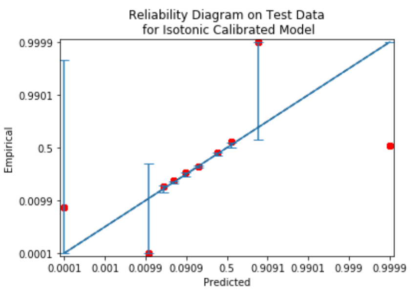
rd = mli.plot_reliability_diagram(y_test_1, testset_iso_probs, scaling='logit', bins=custom_bins_a)
plt.title('Reliability Diagram on Test Data\n for Isotonic Calibrated Model')

The reliability diagram after using isotonic is illustrated here:

V. Conclusion

Overall, we've discoreverd calibration in machine learning which is a very important topic.You can dive deeper with the documents in the reference.And the code above is just some samples to guide you.For more details, please check this github repo

References

[1]. Paper:On Calibration of modern neuron network