Vehicle Insurance Sales [ML Project]

Open-Source Internship opportunity by OpenGenus for programmers. Apply now.

Introduction
Data Description
Data Analysis
Model Building
Evaluation of Signficance
Interpretations and Conclusions
Limitations

Introduction

The research question is what factors influence different types of people to buy auto insurances from a specific company.

The data can be found on Kaggle and contains general information of people the company reached out, where the company collects their potential buyers' gender, age, anual premium etc. and records whether they bought the insurance or not, with 1 being they did, and 0 being they didn't. Upon exploration, variables Gender, Previously_Insured, Vehicle_Age and Vehicle_Damage put significant contributions to the prediction of responses, as explained in the analysis below. The purpose of choosing this topic is to create an ideal model where the company inserts one's information (varaibles as mentioned above), and will be given a prediction of the likliness of that person buying their insurance. This enables the company to eliminate unnecessary follow-ups and sales pursuing those who are less likely to buy insurance, and thus saves both time and resources for actual future clients. The result is important because it not only helps the unsurance company categorize their customers, but also gives its readers a general sense of the relationship between each variable and final response in terms of car insurances. By using a logistic model, I get a better sense as to which variables the company should pay more attention to in order to increase their sellings. I was also able to use a KNN model to locate those who are more likely not interested in buying the insurance. The reason for using logistic and KNN models is that logistic models are specifically designed for binary independent variables, in the case, response = 0 and response = 1, thus I feel like this is the most appropriate model used to predict the results; furthermore, KNN models are easy to train and are good starting points since I would like to separate the possible future customers in to interested/uninterested categories. As a result, the final accuracy rate for both models are approximately 87%, which is fairly accurate and is suitable for predictions.

We will first import the necessary libraries before doing the analysis

import pandas as pd
import numpy as np
import matplotlib.pyplot as plt
import sklearn as sk
import seaborn as sns
from sklearn.metrics import accuracy_score
from sklearn.model_selection import train_test_split
from sklearn.linear_model import LogisticRegression
from sklearn.neighbors import KNeighborsClassifier
from sklearn.feature_selection import RFE

If you don't have any of the libraries, simply run pip install ___ in your command line and install the packages.

Data Description

df = pd.read_csv("insurance_sales_data.csv")
df = df.drop("Unnamed: 0", axis = 1)
df

pic-1
pic-2

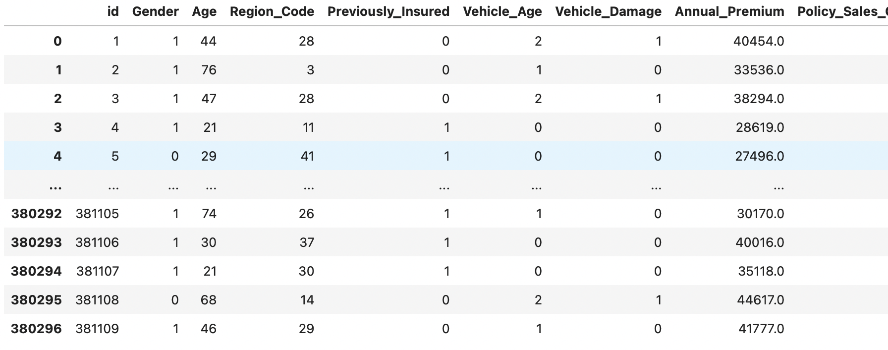
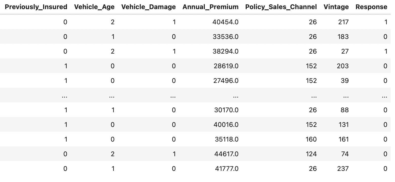
Observations

Each row is a different observation, a customer that purchased or did not purchase the insurance product.

Attributes

id : Unique ID for the customer
Gender : Gender of the customer 1: Male 0: Female
Age : Age of the customer
Region_Code : Unique code for the region of the customer
Previously_Insured : 1 : Customer already has Vehicle Insurance, 0 : Customer doesn't have Vehicle Insurance
Vehicle_Age : Age of the Vehicle 0: less than 1 year , 1: 1-2 years , 2: greater than 1 year
Vehicle_Damage : 1 : Customer got his/her vehicle damaged in the past. 0 : Customer didn't get his/her vehicle damaged in the past.
Annual_Premium : The amount customer needs to pay as premium in the year
Policy_Sales_Channel : Anonymized Code for the channel of outreaching to the customer ie. Different Agents, Over Mail, Over Phone, In Person, etc.
Vintage : Number of Days, Customer has been associated with the company
Response : 1 : Customer is interested, 0 : Customer is not interested

Data analysis

We will be doing some exploratory data anlaysis before diving in into the model building part

print("mean age for the dataset is " + str(round(df.Age.mean())))
print("median age for the dataset is " + str(round(df.Age.median())))

Mean age for the dataset is 39
Median age for the dataset is 36

a18t30 = df[(df.Age >= 18) & (df.Age < 30)]
a30t40 = df[(df.Age >= 30) & (df.Age < 40)]
a40t50 = df[(df.Age >= 40) & (df.Age < 50)]
a50t60 = df[(df.Age >= 50) & (df.Age < 60)]
a60t70 = df[(df.Age >= 60) & (df.Age < 70)]
a70t80 = df[(df.Age >= 70) & (df.Age < 80)]
a80t90 = df[(df.Age >= 80) & (df.Age < 90)]
labels = ['18 to 30', '30 to 40', '40 to 50', '50 to 60', '60 to 70', '70 to 80', '80 to 90']
sizes = [a18t30.id.size, a30t40.id.size, a40t50.id.size, a50t60.id.size, a60t70.id.size, a70t80.id.size, a80t90.id.size]
fig1, ax1 = plt.subplots()
ax1.pie(sizes, labels=labels, autopct='%1.1f%%', shadow=True)
ax1.axis('equal')
plt.title("Distrbution of Different Age Groups in the Dataset")
plt.show()

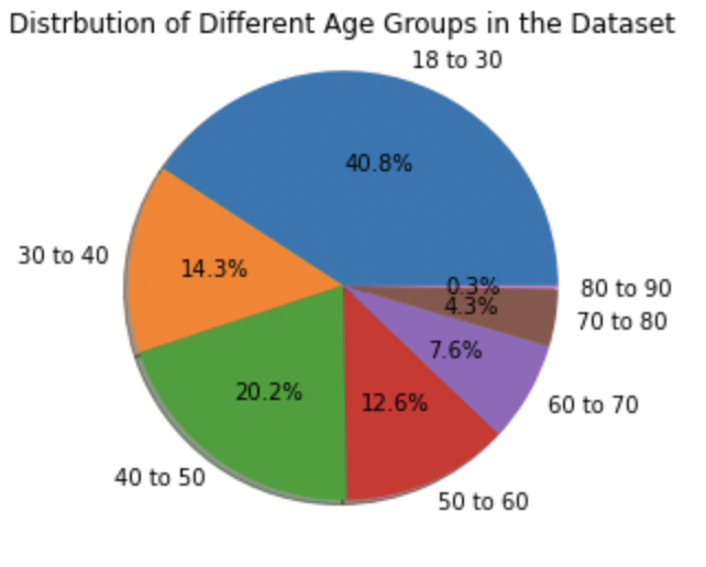
We can see that in the dataset, most of the data comes from the age group of 18 to 30.

a18t30r = a18t30[a18t30.Response == 1].id.size / a18t30.id.size
a30t40r = a30t40[a30t40.Response == 1].id.size / a30t40.id.size
a40t50r = a40t50[a40t50.Response == 1].id.size / a40t50.id.size
a50t60r = a50t60[a50t60.Response == 1].id.size / a50t60.id.size
a60t70r = a60t70[a60t70.Response == 1].id.size / a60t70.id.size
a70t80r = a70t80[a70t80.Response == 1].id.size / a70t80.id.size
a80t90r = a80t90[a80t90.Response == 1].id.size / a80t90.id.size
labels = ['18 to 30', '30 to 40', '40 to 50', '50 to 60', '60 to 70', '70 to 80', '80 to 90']
rates = [a18t30r, a30t40r, a40t50r, a50t60r, a60t70r, a70t80r, a80t90r]
plt.bar(labels, rates, color='green')
plt.title("Percentage of People in the Age Groups buying the Insurances")
plt.xlabel("Age")
plt.ylabel("Perecent of People Purchasing Insurance")

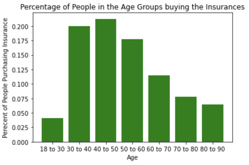
We see that for it is most likely for the age group of 40 to 50 to purchase the insurances

switch_company = df[(df.Previously_Insured == 1) & (df.Response == 1)].id.size
newbie = df[(df.Previously_Insured == 0) & (df.Response == 1)].id.size
no_longer = df[(df.Previously_Insured == 1) & (df.Response == 0)].id.size
never_been = df[(df.Previously_Insured == 0) & (df.Response == 0)].id.size
names = ['switched insurance companies', 'first time insured', 'did not switch company', 'never insured']
countt = [switch_company, newbie, no_longer, never_been]
plt.barh(names, countt, color = 'green')
plt.xlabel('amount of people')
plt.ylabel('prospective categories for Previously_Insured and Response')
plt.title('previously insured and response to buying insurance')

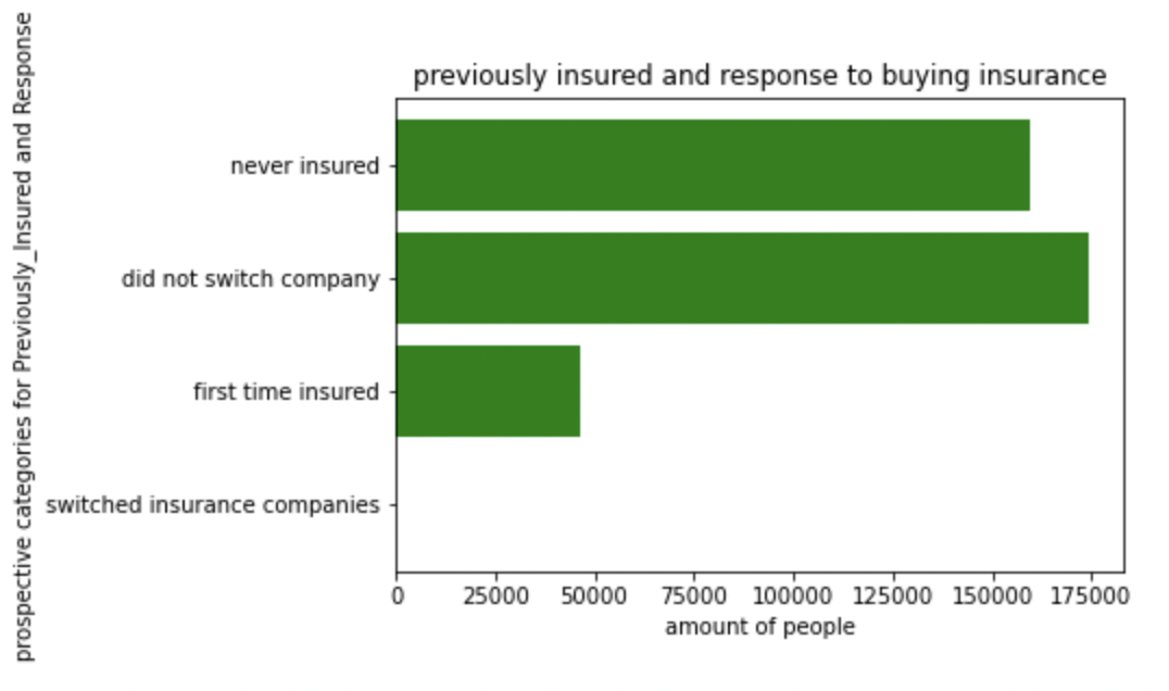
As shown on the graph, the majority of customers prefer to stay with the current insurance company if they have one. We can see that the number of customers who switched companies is approximately zero (or super low). It also stuck out that lots of people prefer to not insure their car at all, corroborated by the first bar labeled 'never insured' on the graph.

Now we will build the correlation map and see what variables have high corelations

X=df.drop(['id','Policy_Sales_Channel'], axis=1)
corr = X.corr()

fig = plt.figure()
ax = fig.add_subplot(111)
ax.matshow(corr)

ax.set_xticks(range(len(corr.columns)))
ax.set_xticklabels(corr.columns)
for tick in ax.get_xticklabels():
        tick.set_rotation(45)

ax.set_yticks(range(len(corr.columns)))
ax.set_yticklabels(corr.columns)

fig.set_size_inches(20, 20)
plt.show()

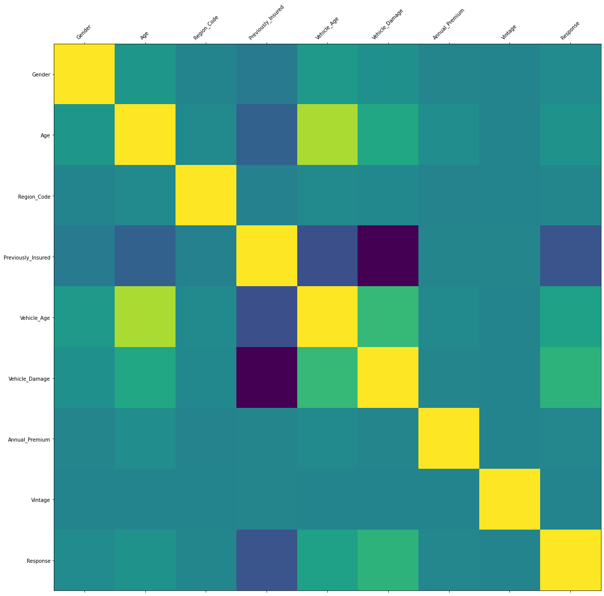
Vehicle Damage and Previously Insured has a deep color according to the correlation map

We are aware of the dataset identities, and now we will start building models to predict the insruance sales.

Model building

We will first build a logistic model to fit the data. Logistic models predicts a value between 1 and 0 and we can use that to predict the different classes.

X = df.drop(['id', 'Response'], axis=1)
Y = df['Response']

X_train, X_test, Y_train, Y_test = train_test_split(X, Y, test_size=0.20, random_state=42)
modellog = LogisticRegression(max_iter=10000)
rfe = RFE(modellog)
logistic_model = rfe.fit(X_train, Y_train)

logistic_model.fit(X_train, Y_train)

pred_train = logistic_model.predict(X_train)
pred_test = logistic_model.predict(X_test)

print("Test Accuracy: ", accuracy_score(Y_test, pred_test))
print("Training Accuracy: ", accuracy_score(Y_train, pred_train))

And we will see that
Test Accuracy: 0.8782145674467525
Training Accuracy: 0.877049799991454

Let's also examine what variables the logistic regression chose

print("Selected Features: %s" % logistic_model.support_)
for i in range(len(X.columns)):
    if (logistic_model.support_[i]):
        print(X.columns[i])

Variables Choosen by the model:
Gender
Previously_Insured
Vehicle_Age
Vehicle_Damage

Now, we will build the KNN model:

x = df[['Gender', 'Age', 'Vehicle_Age', 'Previously_Insured', 'Vehicle_Damage', 'Annual_Premium']]
y = df['Response'].values
x_train, x_test, y_train, y_test = train_test_split(x, y, test_size = 0.20, random_state = 115)
knn = KNeighborsClassifier(n_neighbors = 4)
knn.fit(x_train, y_train)
print("accuracy of knn model: ", knn.score(x_test, y_test))

The accuracy score of the KNN model is 0.8667104917170655

Evaluation of the Significance

First, we will look at the logistic model

import statsmodels. api as sm  
X = df.drop(['id', 'Age','Region_Code','Annual_Premium','Policy_Sales_Channel','Vintage','Response'], axis=1)
Y = df['Response']
log_reg = sm.Logit(Y, X).fit() 
print(log_reg.summary())

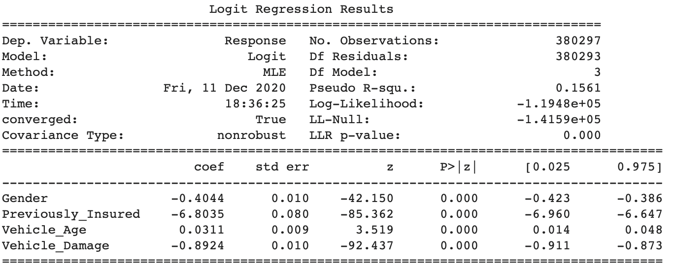
for gender variable, it has a z score of -42.15 and a p-value less than 0.001, which means it is significant in prediciting whether a customer will purchase the product or not. It applies to the previously_Insured variable, Vehicle_Age variable, Vehicle_Damage variable as well, we see that the p-values are all less than 0.001 which means that feature selection is successful in the data analysis section. All the selected variables are significant in predicting the response variable through a logistic regression.

Now, we will check out the KNN model

from sklearn.metrics import classification_report, confusion_matrix
y_pred = knn.predict(x_test)
print(confusion_matrix(y_test, y_pred))
print(classification_report(y_test, y_pred))

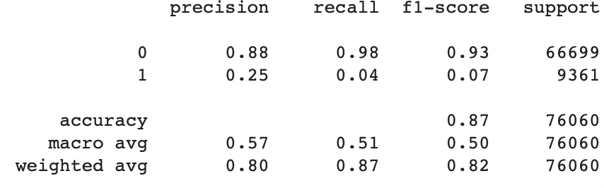
For the responses, 0 indicates the customer won't buy the insurance, and 1 being that they will. We can see from the precision score that 88% of the '0' responses were predicted correctly, however only 25% of the predicted '1' responses were accurate. Arguably a large sum of the data consists of customers who indicated that they won't buy the insurance, thus the weighted average precision is relatively high, 80%. For a KNN model we can't explicitly see how each of the variables contribute their significance and prediction accuracy.

Interpretations and Conclusions

Logistic Model

From the logistic model we can see that the features selected are Gender, Previously_Insured, Vehicle_Age and Vehicle_Damage. The features are selected through the rfe(recursive feature elimination) process.

Thus the weakest varaibles are dropped, and variables with collinearities are dropped. Interestingly enough, they are all categorical variables. The accuracy score I got from the model is 87% which I believe is a very high score for predicting whether a customer will purchase a product or not. If we can accurately predict whether customers will purchase the product 87% of the time, companies can better allocate resources for better marketing strategies.

Companies can focus on specific Gender, Previously Insured status, Vehicle Age status and Vehicle Damage status to better target which customers are more likely to purchase their products. For Gender, we can see that the coefficient of the logistic model if -0.4044, which means being female will make the purchasing of the product more likely. The reason for this might be in a family, the wife might have more say in buying power. As a result, more females will make the decision of whether or not the insurance should be bought or not. So marketing strategies for this company should target females.

For the previously Insured variable, we see that not being previously insured at another company is very important in predicitng whether the customer will buy the insruance product. The coefficient is -6.8 which is very high compared to the other significant variables. The reason for this might be it is unlikely for individuals to switch insurance companies once the individual is willing to buy an isurance product already.

For the Vehicle_Age variable, we see that it has a coefficient of 0.0311 which is not very high, but its p-value determines that it is significant. It is more liekly for individuals that owns vehicle that has a higher vehicle age to buy the product.

Since vehicle age is high, it is more likely for the vehicle to run into problems, therefore an insurance might be needed. For the vehicle damage variable, it is more likely for individuals that own cars that didn't havev vehicle damage before to buy the insurance product. This is probably because if individual's car is damaged, it is pointless now to buy the product and also the product will be much more pricier for the individual due to how insurance works.

So according to the logistic model, in order for the company to sell their product better, they should focus on the following variables: Gender, Prevviously_Insured, Vehicle_Age and Vehicle_Damage.

KNN Model

The KNN model is used to sort potential buyers into two categories, (rather than for prediction). K value is set to 4, meaning that 4 of the closest training samples to the point is selected then placed into one of the two categories.

There are a number of ways to find this number, and first tried the square root of the number of observations in the training set (552). However for this number it is found that the prediction for response = 1 is 0% accuracy.

After that I started from 1 and continued to go up, realizing that 4 gives the best general accuracy percentage.

For this KNN model, the independent variables chosen to predict the response are Gender, Age, Vehicle_Age, Previously_Insured, Vehicle_Damage, and Annual_Premium. Age and Annual_Premium are quantitative data while all the other ones are categorical.

It is known that KNN models work better with quantitative data, and with 33% of selected variables being quantitative, the accuracy score is 87%, which is still relatively high. I dropped features id, region_code, policy_sales_channel and vintage because there's no way for me to make sense of what those numbers mean (i.e. I don't know what each represent).

However, as seen from the confusion matrix and classification report, this model predicts the likelihood of a potential customer turning down the insurance offer as opposed to buying it. Out of 66699 test cases with response '0', 65521 cases were indeed tested accurate, and out of 9361 test cases with response '1', only 322 cases turned out to be true, summing up to a total of 76060 test cases.

This further corroborates the finding that while I can use this model to accurately classify customers who are not interested, it is not the best model to test that they are.

Limitations

Different Age group might lead to different groups with different amount of wealth. Maybe it will be shown that older people are more likely to purchase the insurance, but it might not be a causation, it can just be a correlation.

Information on exactly what each different number for policy sales channels stand for is not provided, but it is definitely an important reason for why people choose to purchase insurances.

For each columns, if one speicfic value appears too many times, the analysis might be inaccurate because the model built might not predict the values with less appearnces accurately. So for example, if for vehicle age, only 100 datasets for vehicles under 1 year is avilable, then the model for predicting the response might not be accurate for that specific feature.

If there are not enough data for a certain category, we might not be able to make an accurate prediction.