Assembly Line Scheduling using Dynamic Programming

In an product industry, produts are produced using assembly lines. Multiple lines are worked together to produce a useable product and completed useable product exits at the end of the line.

For making a product in the optimal time we should choose the optimised assembly line from a station so that a company can make product in the best utilized time.

Problem Statement

The main goal of solving the Assembly Line Scheduling problem is to determine which stations to choose from line 1 and which to choose from line 2 in order to minimize assembly time.

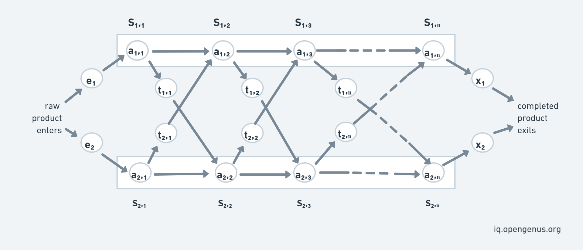
In the above the diagram we have two main assembly line consider as LINE 1 and LINE 2. Parameters are:

• S[i,j]: The jth station on ith assembly line
• a[i,j]: Time required at station S[i,j], because every station has some dedicated job that needs to done.
• e[i]: Entry time of product on assembly line i [here i= 1,2]
• x[i]: Exit time from assembly line i
• t[i,j]: Time required to transit from station S[i,j] to the other assembly line.

Hence, the input consist of:

S[i,j] = j-th station on i-th assembly line
a[i,j] = Time required do task at station S[i,j]
e[i] = Entry time of product on assembly line i [here i= 1,2]
x[i] = Exit time from assembly line i
t[i,j] = Time required to transit from station S[i,j] to the other assembly line

Normally, when a raw product enters an assembly line it passes through through that line only. Therefore, the time to go from one station to another station of same assembly line is negligible but to pass a partially completed product from one station of a line to other station of another line a t[i,j] is taken.

It is a optimization problem in which we have to optimized the total assembly time. To solve the optimization problem we make use of Dynamic Programming. To solve with DP we will see how it have Overlapping Subproblem and Optimal Substructure.

Consider that f[i,j] denotes the fastest time taken to get the partially completed product from starting point through ith line and jth station.

The DP structure is as follows:

f[i, j] = minimum time taken to get product from starting point through i-th line and j-th station

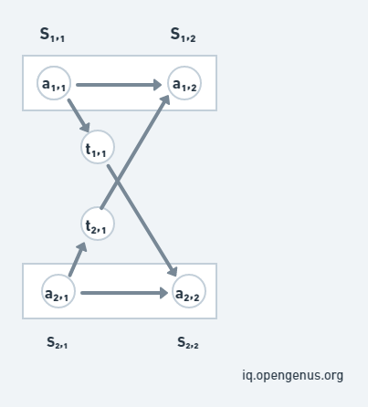
Consider the above image, we can reach S[1,j] in two ways, either from station S[1,j-1] or from station S[2,j-1]. We have to find the minimum time from both the ways:-

• Time taken to reach from 1st line will be, f[1,j-1] + a[1,j].
• Time taken to reach from 2nd line will be, f[2,j-1] + t[2,j-1] + a[1,j].

If the partial product comes from S[2,j-1], additionally it incurs the transfer cost to change the assembly line (like t[2,j-1]).

Note that, minimum time to leave S1[j-1] and S2[j-1] have already been calculated.

We can notice from this example that the approach is using the already solved time from f[1,j-1], so the Overlapping Subproblem is used. And to find the fastest way through station j, we solve the sub-problems of finding the fastest way through station j-1 which is the Optimal Substructure.

Breaking in smaller sub-problems

We will use the Bottom-Up approach to find the minimum time to complete a product and for that consider f1 & f2 be time taken from line 1 & 2 respectively and 'e'
& 'x' are the entry & exiting time respectively. The following are the cases that we will use:

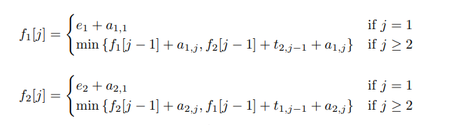
• Base-Case: At station 1 at partial product directly comes from entry point, therefore f1[1]= e1 + a[1,1] and f2[1]= e2 + a[2,1].
• For calculating time to reach at jth station from line 1 we will find the optimal time as we discussed above, f[1,j]= min{f1[j-1]+a[i,j], f2[j-1]+t[2,j-1]+a[1,j]}
• The optimized or fastest time to exit a completed product will be f optimal= min{f1[n] + x1, f2[n] + x2}.

We need two tables to store the partial results calculated for each station in an assembly line. The table will be filled in a bottom-up fashion.

The recursion to reach the station j in assembly line i are as follows:

Pseudo Code for Assembly Line Scheduling

where 'a' denotes the assembly costs, 't' denotes the transfer costs, 'e' denotes the entry costs, 'x' denotes the exit costs and 'n' denotes the number of assembly stages.

START
f1[1] = e1 + a1,1
f2[1] = e2 + a2,1
    for j = 2 to n
        if ((f1[j − 1] + a1,j ) ≤ (f2[j − 1] + t2,j−1 + a1,j )) then
            f1[j] = f1[j − 1] + a1,j
        else
            f1[j] = f2[j − 1] + t2,j−1 + a1,j
        if ((f2[j − 1] + a2,j ) ≤ (f1[j − 1] + t1,j−1 + a2,j )) then
            f2[j] = f2[j − 1] + a2,j
        else
             f2[j] = f1[j − 1] + t1,j−1 + a2,j
    end for
    if (f1[n] + x1 ≤ f2[n] + x2) then
        fopt = f1[n] + x1
    else
        fopt = f2[n] + x2
END

Implementation in C++

Following is our C++ implementation of solving the Assembly Line Scheduling problem using Dynamic Programming:

// A C++ program to find minimum possible 
// time to complete a product 
#include <bits/stdc++.h>
using namespace std;
 
int productAssembly(int a[][5], int t[][4], int e[2], int x[2]) 
{ 
    int f1[5], f2[5]; 
 
    // time taken to reach first station at line 1 
    f1[0] = e[0] + a[0][0]; 
     
    // time taken to reach first station at line 2 
    f2[0] = e[1] + a[1][0]; 
 
    // fill tables f1[] and f2[] using the 
    // given recursive relations 
    for(int j = 1; j< 5; j++) 
    { 
        f1[j] = min(f1[j - 1] + a[0][j], 
                    f2[j - 1] + t[1][j-1] + a[0][j]); 
        f2[j] = min(f2[j - 1] + a[1][j],
                    f1[j - 1] + t[0][j-1] + a[1][j]); 
    } 
 
    // Consider exit times and return minimum 
    return min(f1[4] + x[0], f2[4] + x[1]); 
} 
 
// Driver Code
int main() { 
    int a[2][5] = { {8, 10, 4, 5, 9}, 
                    { 9, 6, 7, 5, 6} }; 
    int t[2][4] = { {2, 3, 1, 3}, 
                    {2, 1, 2, 2} }; 
    int e[2] = {3, 5};
    int x[2] = {2, 1}; 
 
    cout<<"Optimal Time for completing the product is: "<<productAssembly(a, t, e, x); 
 
    return 0; 
} 

Output:
Optimal Time for completing the product is: 37

The pictorial view of the Question is this:

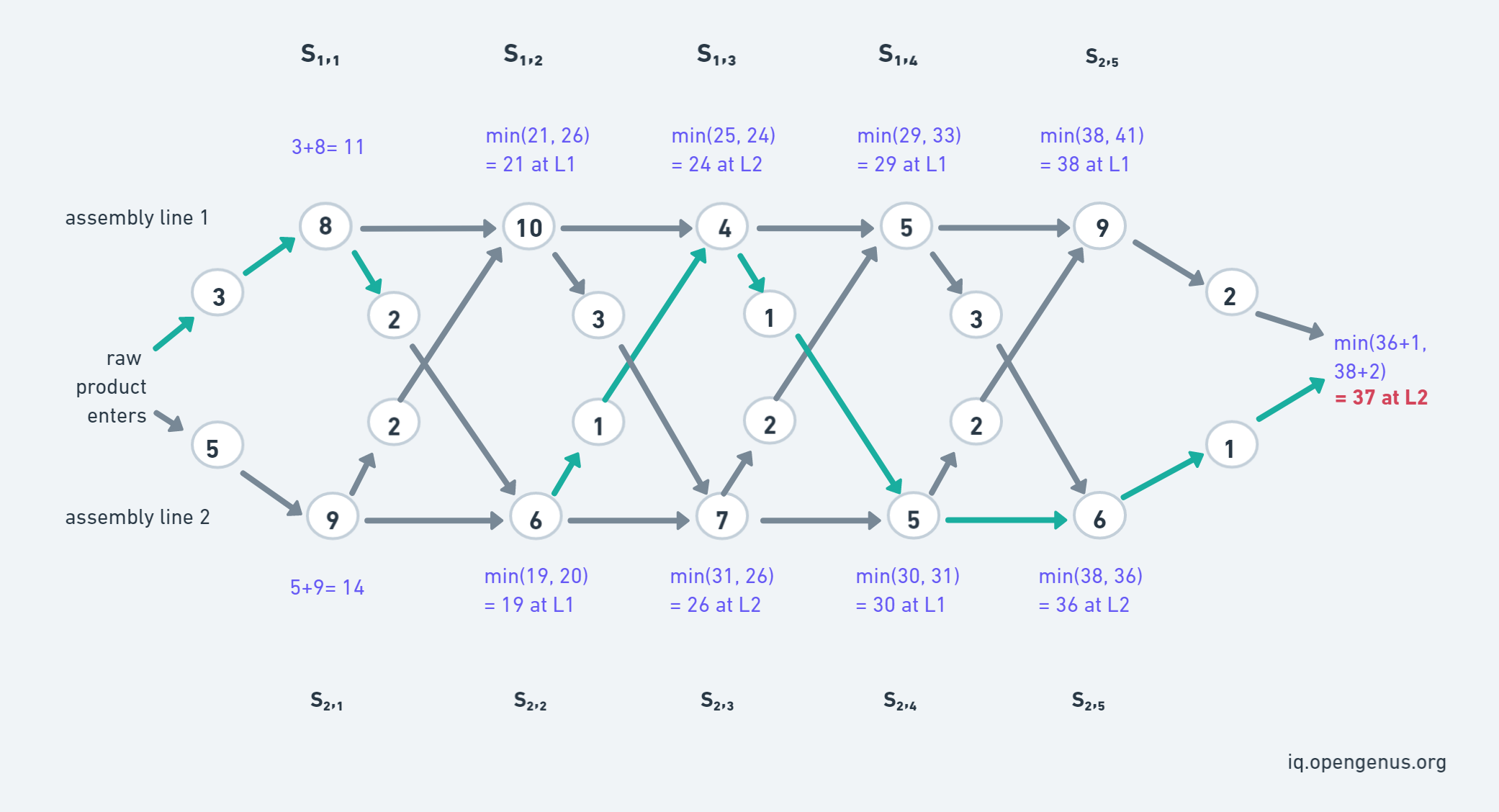
The pictorial view of the dp array that store the partial results calculated for each station in an assembly line. And line number table that help you to understand from which line the optimized solution comes from (it is for explanation only).

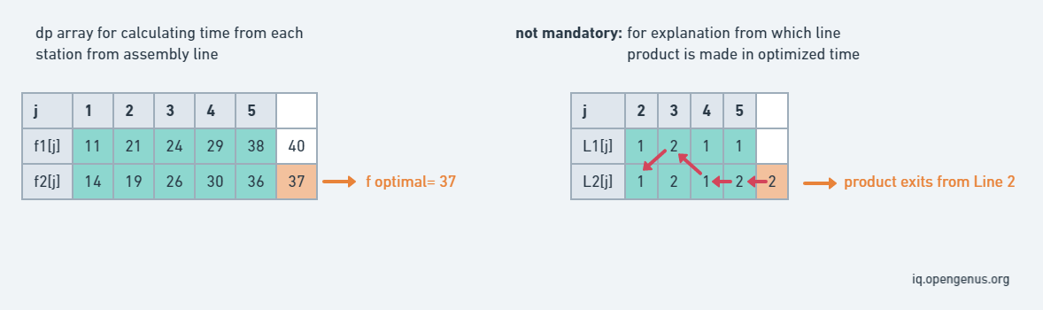
Workflow of solution

• As a[2][5] defined in code denotes that we have 2 assembly line and 5 stations. Then f1[0] and f2[0] is defined by adding entry time (e[i]) and first station time.
• Then applies the recursive solution for n station points, the l1[j] denotes from which assembly line partial product comes from.
• We will choose the optimized time by calculating minimum time by continuing on the same assembly time or by changing the assembly line (if line changed then t[i][j-1] time will also be added).
• At last f optimal is calculated by minimum of the time at the last station, added with the exiting time of the line from which the product exit.

Time Complexity

As the dp tabulation array is used and the 'n' iteration is done to store the optimal time in the array, therefore the time complexity of the above Dynamic Programming implementation of the assembly line scheduling is O(n).
We are storing the optimal time taken to pass through station in an array, therefore the space complexity will be O(n).