Kolmogorov-Arnold Networks

Open-Source Internship opportunity by OpenGenus for programmers. Apply now.

Kolmogorov-Arnold Networks (KANs) have emerged as a promising  advancement in the field of neural networks, offering enhanced  interpretability, efficiency, and adaptability compared to traditional  architectures like the Multi-Layer Perceptron (MLPs).

Brief intro to MLPs

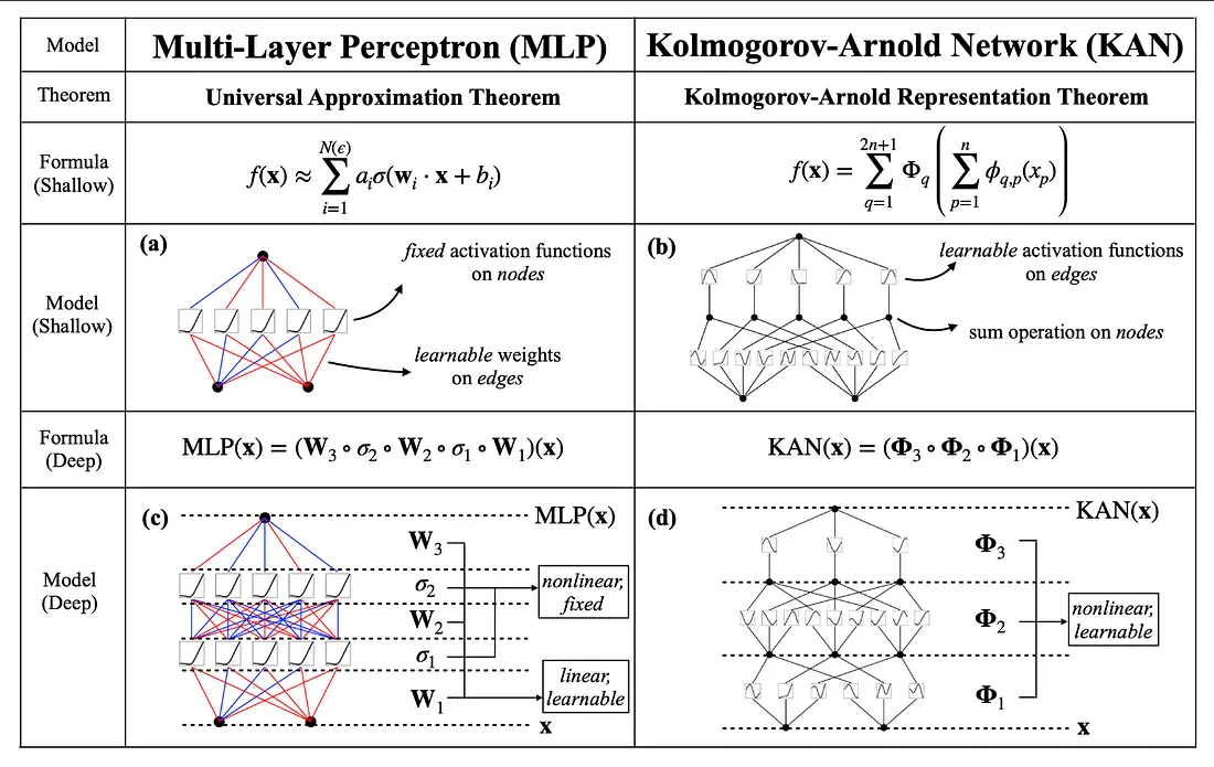
MLPs, or Multi-Layer Perceptrons, are an important part of current neural networks. They are made up of layers of nodes, or "neurons," that are linked to each other and are meant to learn from data and approximate complex, nonlinear functions. Each neuron uses a set activation function on the weighted sum of its inputs to turn input data into the output that is wanted. This is done by breaking down the input data into many smaller pieces.

KANs

Andrey Kolmogorov and Vladimir Arnold came up with the Kolmogorov-Arnold representation theorem, which says that any multivariate continuous function can be shown as a finite combination of continuous functions of a single variable and the addition operation. This theory says that complicated functions with a lot of dimensions can be broken down into simpler functions with only one variable.

Unlike traditional MLPs that use fixed activation functions at each node or neuron, KANs employ learnable activation functions on the edges (weights) of the network. KANs have no linear weights at all, what this means is that every weight parameter is replaced by a univariate function parametrized as a spline. This allows KANs to adaptively learn the best functions to apply during  training, enhancing flexibility and pattern capturing ability.

But, what is a spline? The initial implementation of KANs used B-Splines as their foundation, and here's a brief overview from wikipedia:

"In the mathematical subfield of numerical analysis, a B-spline or basis spline is a spline function that has minimal support with respect to a given degree, smoothness, and domain partition."

Which in essence is the method in which KANs approximate functions.

However, there are multiple ways of approximating functions, there are Polinomials (Chebyshev, Jacobi, Orthogonal, and more), Gaussian Radial Basis Functions (RBFs), Fourier, Wavelets, etc., so the jury is still out on what is the best and most efficient way to implement KANs. There's also ReLU KANs, K-A Transformers, K-A CNNs, Graph KANs, and a lot more.

Math

Here's a quick run-down of what's happening at the original B-Spline implementation:

The Kolmogorov-Arnold representation theorem states that if \( f \) is a multivariate continuous function on a bounded domain, then it can be written as a finite composition of continuous functions of a single variable and the binary operation of addition.

For a smooth function \( f: [0,1]^n \to \mathbb{R} \), it can be expressed as:

\[ f(x) = f(x_1,...,x_n) = \sum_{q=1}^{2n+1}\Phi_q\left(\sum_{p=1}^n \phi_{q,p}(x_p)\right) \]

Coding a KAN

Now, we'll follow the code found in the official documentation (hellokan.ipynb).

To initialize a KAN:

from kan import *
torch.set_default_dtype(torch.float64)

device = torch.device('cuda' if torch.cuda.is_available() else 'cpu')
print(device)

# create a KAN: 2D inputs, 1D output, and 5 hidden neurons. cubic spline (k=3), 5 grid intervals (grid=5).
model = KAN(width=[2,5,1], grid=3, k=3, seed=42, device=device)

We create a basic dataset to work with:

from kan.utils import create_dataset
# create dataset f(x,y) = exp(sin(pi*x)+y^2)
f = lambda x: torch.exp(torch.sin(torch.pi*x[:,[0]]) + x[:,[1]]**2)
dataset = create_dataset(f, n_var=2, device=device)
dataset['train_input'].shape, dataset['train_label'].shape

We plot the KAN at initialization:            ‌

# plot KAN at initialization
model(dataset['train_input']);
model.plot()

We train the KAN with sparsity regularization:

# train the model
model.fit(dataset, opt="LBFGS", steps=50, lamb=0.001);

We plot the trained KAN:

model.plot()

We prune the KAN and replot:

model = model.prune()
model.plot()

We continue training and replotting:

model.fit(dataset, opt="LBFGS", steps=50);

We refine the model:

model = model.refine(10)

We continue training and replotting on the refined model:

model.fit(dataset, opt="LBFGS", steps=50);

We can automatically or manually set activation functions to be symbolic:

mode = "auto" # "manual"

if mode == "manual":
    # manual mode
    model.fix_symbolic(0,0,0,'sin');
    model.fix_symbolic(0,1,0,'x^2');
    model.fix_symbolic(1,0,0,'exp');
elif mode == "auto":
    # automatic mode
    lib = ['x','x^2','x^3','x^4','exp','log','sqrt','tanh','sin','abs']
    model.auto_symbolic(lib=lib)

We can continue training for machine precision:

model.fit(dataset, opt="LBFGS", steps=50);

And finally, we can obtain the symbolic formula:

from kan.utils import ex_round

ex_round(model.symbolic_formula()[0][0],4)

If you want to learn more, here is the official pykan repo (MIT Licence), where you can find more examples, tutorials, and more information.

Further reading

As we mentioned before, KANs are still relatively new and thus, unexplored. There have been many advancements and insights from the community, and from the original authors as well. You can find a lot more information on the following links:

Original Paper

Update from original authors (improvements and developments)

Code from original authors (MIT Licence)

KAN or MLP: A Fairer Comparison

Rethinking the Function of Neurons in KANs (Using mean instead of sum)

Awesome KAN GitHub Repo (a lot of info on KANs and their uses, MIT Licence)