Open-Source Internship opportunity by OpenGenus for programmers. Apply now.
In this article, we will understand and implement both versions of the Brandes algorithm in python. To be specific, Edge and Vertex betweenness Centrality computation for the unweighted graph as proposed in the original publication. In addition, we try a modified version that uses Dijkstras algorithm for weighted graph variants with preliminary verification.
table of contents
- Introduction
- Pseudo code
- Code Implementation
- Pros and Cons
- Creative weighted modification
- Review and References
Introduction
Graphs are elegant mathematical representations used to model sophisticated real-world structures and processes. Some components(Vertice/Edge) of the graph are of higher interest because of their relative orientation within the graph. We are entailed to generate a measure that quantifies the significance because of their correlated applications. This measure is also called Betweenness Centrality and depending on the component of interest it is prefixed with Vertex or Edge.
For quite some time(>50 years) researchers were keen on addressing the various questions in regard to graph algorithms and also trying to improve the existing methods. Following the same came a paper titled "A Faster Algorithm for Betweenness Centrality" by Ulrik Brandes published in 2001 which highlighted an improved Vertex and Edge betweenness Centrality computation algorithm that would then go on to be called the Brandes algorithm.
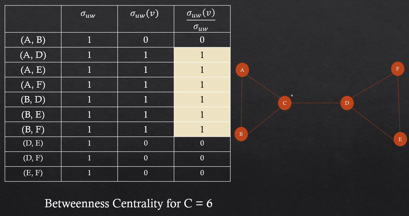
Most contemporary graph algorithms are fundamentally intuitive. To substantiate, the conceptual idea behind betweenness centrality is to capture the significance by figuring out the portion of times in which the shortest paths between pairs of vertices is individually and directly affected by the Vertex or Edge in interest.
For example consider this graph to work with,

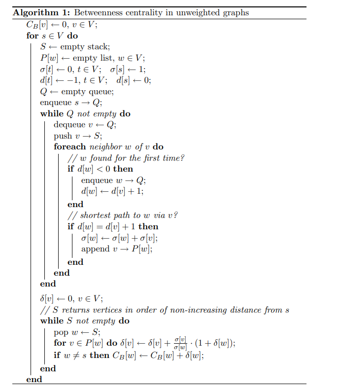
Pseudo-Code
The pseudo-code for the algorithm derived from the above-mentioned paper is as follows,

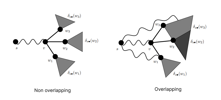
The logic to handle overlapping paths can be understood from the following figure,

for the non-overlapping case the definition is "If there is exactly one shortest path from s ∈ V to each t ∈ V, the dependency of s on any v ∈ V obeys"

and for the overlapping case, the definition is "fractions of the dependencies on
successors are propagated up along the edges of the directed acyclic graph
of shortest paths from the source tain both v and e"

The proofs and subproofs are omitted here but can be found in the references from the paper itself.
Code Implementation
The code illustrated here is derived form here
Edge Betweenness Centrality computation function
def brandes(V, A):
    "Compute betweenness centrality in an unweighted graph."
    # Brandes algorithm
    # see http://www.cs.ucc.ie/~rb4/resources/Brandes.pdf
    C={}
    for v in V:
        for e in A.keys():
            C[(v,e)] = 0
    for s in V:
        S = []
        P = dict((w,[]) for w in V)
        g = dict((t, 0) for t in V); g[s] = 1
        d = dict((t,-1) for t in V); d[s] = 0
        Q = deque([])
        Q.append(s)
        while Q:
            v = Q.popleft()
            S.append(v)
            for w in A[v]:
                if d[w] < 0:
                    Q.append(w)
                    d[w] = d[v] + 1
                if d[w] == d[v] + 1:
                    g[w] = g[w] + g[v]
                    P[w].append(v)
        e = dict((v, 0) for v in V)

        while S:
            w = S.pop()
            for v in P[w]:
                e[v] = e[v] +  g[w]* (1 + (e[w]/g[w]))
                C[(v, w)] = C[(v, w)] + g[v]*(e[w]/g[w] +1)

    return C
likewise,
Vertex Betweenness Centrality computation function
def brandes(V, A):
    "Compute betweenness centrality in an unweighted graph."
    # Brandes algorithm
    # see http://www.cs.ucc.ie/~rb4/resources/Brandes.pdf
    C = dict((v,0) for v in V)
    for s in V:
        S = []
        P = dict((w,[]) for w in V)
        g = dict((t, 0) for t in V); g[s] = 1
        d = dict((t,-1) for t in V); d[s] = 0
        Q = deque([])
        Q.append(s)
        while Q:
            v = Q.popleft()
            S.append(v)
            for w in A[v]:
                if d[w] < 0:
                    Q.append(w)
                    d[w] = d[v] + 1
                if d[w] == d[v] + 1:
                    g[w] = g[w] + g[v]
                    P[w].append(v)
        e = dict((v, 0) for v in V)
        while S:
            w = S.pop()
            for v in P[w]:
                e[v] = e[v] + ((g[v]/g[w]) * (1 + e[w]))
            if w != s:
                C[w] = C[w] + e[w]

    for v in V:
        C[v] = C[v] / 2
    return C
Pros and Cons
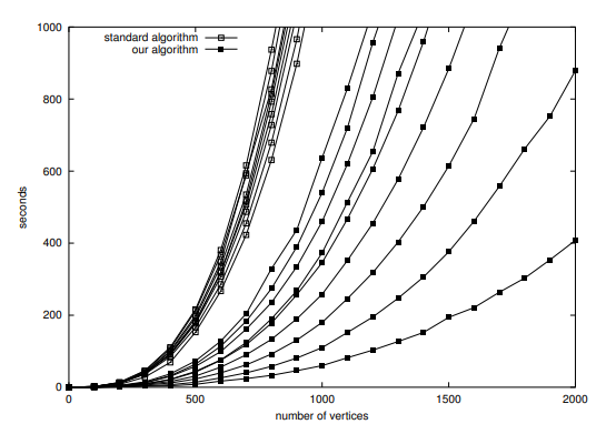
The performance results highlighted in the paper are,

Pros for Vertex Betweenness Centrality:
- The Brandes algorithm is widely regarded as one of the most efficient algorithms for computing vertex betweenness centrality, and it has been used in many studies to analyze large-scale networks.
- The algorithm can handle weighted graphs, directed graphs, and graphs with negative edge weights. but only un-weighted graphs native implementation
- The output of the algorithm can be easily interpreted and can provide insights into the most important nodes in the network.
Cons for Vertex Betweenness Centrality:
- The algorithm requires a large amount of memory to store the data structures used during computation, which can make it impractical to use on very large graphs.
- The algorithm has a worst-case time complexity of O(nm), which can be slow for very large graphs.
- The algorithm is not well-suited for computing vertex betweenness centrality in dynamic networks, where the network structure changes over time.
Pros for Edge Betweenness Centrality:
- The Brandes algorithm can also be used to compute edge betweenness centrality, which can provide insights into the most important edges in the network.
- The algorithm is also efficient for computing edge betweenness centrality, and it can be used on large-scale networks.
- The output of the algorithm can be easily interpreted and can provide insights into the most important edges in the network.
Cons for Edge Betweenness Centrality:
- The algorithm requires a large amount of memory to store the data structures used during computation, which can make it impractical to use on very large graphs.
- The algorithm has a worst-case time complexity of O(nm), which can be slow for very large graphs.
- The algorithm may not be well-suited for computing edge betweenness centrality in certain types of networks, such as dense networks or networks with a large number of cycles.
Creative weighted modification
The use of naive Dijkstra's algorithm to handle the weighted components has been employeed in the following code,
def dijsktra(graph, source, destination):
    path = {}
    adj_node = {}
    queue = []

    for node in graph:
        path[node] = float("inf")
        adj_node[node] = None
        queue.append(node)

    path[source] = 0
    while queue:
        # find min distance which wasn't marked as current
        key_min = queue[0]
        min_val = path[key_min]
        for n in range(1, len(queue)):
            if path[queue[n]] < min_val:
                key_min = queue[n]
                min_val = path[key_min]
        cur = key_min
        queue.remove(cur)
        # print(cur)

        for i in graph[cur]:
            alternate = graph[cur][i] + path[cur]
            if path[i] > alternate:
                path[i] = alternate
                adj_node[i] = cur


    x = destination
    path = [destination]
    while True:
        x = adj_node[x]
        if x is None:
            break
        path.append(x)
    path.reverse()

    return path
along with parallel component function for vertex and edge betweenness centrality
def vertex_betweenness_centrality(G):
    n_v =len(G)
    counts = [0]*n_v

    for start in range(1, n_v+1):
        for end in range(1, n_v+1):
            if(start!=end):
                path = dijsktra(G, start, end)
                lp = len(path)
                if lp > 2:
                    for idx in range(1, lp-1):
                        element = path[idx]
                        # if element == 1:
                        #     print(path)
                        counts[element-1] += 1

    counts = [i / 2 for i in counts]
    Total = sum(counts) + n_v
    BC = [i / Total for i in counts]
    vertex = range(1, n_v+1)

    VBC = pd.DataFrame({'Vertex' : vertex, 'Counts' : counts,'Betweenness Centrality' : BC}, columns=['Vertex','Counts','Betweenness Centrality'])

    return VBC

def edge_betweenness_centrality(G):
    n_v = len(G)
    sum = 0
    for i in range(1, n_v+1):
        sum += len(G[i])
    n_e = int(sum/2)
    counts = [0]*n_e

    for start in range(1, n_v+1):
        for end in range(1, n_v+1):
            if(start!=end):
                path = dijsktra(G, start, end)

                for i in range(len(path)-1):
                    elm1 = path[i]
                    elm2 = path[i+1]
                    if( ((elm1 == 1) and (elm2 == 2)) or ((elm1 == 2) and(elm2 == 1)) ):
                        counts[0] += 1
                    if( ((elm1 == 1) and (elm2 == 3)) or ((elm1 == 3) and(elm2 == 1)) ):
                        counts[1] += 1
                    if( ((elm1 == 3) and (elm2 == 2)) or ((elm1 == 2) and(elm2 == 3)) ):
                        counts[2] += 1
                    if( ((elm1 == 4) and (elm2 == 2)) or ((elm1 == 2) and(elm2 == 4)) ):
                        counts[3] += 1
                    if( ((elm1 == 3) and (elm2 == 4)) or ((elm1 == 4) and(elm2 == 3)) ):
                        counts[4] += 1
                    if( ((elm1 == 3) and (elm2 == 5)) or ((elm1 == 5) and(elm2 == 3)) ):
                        counts[5] += 1
                    if( ((elm1 == 4) and (elm2 == 5)) or ((elm1 == 5) and(elm2 == 4)) ):
                        counts[6] += 1
                    if( ((elm1 == 4) and (elm2 == 6)) or ((elm1 == 6) and(elm2 == 4)) ):
                        counts[7] += 1
                    if( ((elm1 == 5) and (elm2 == 6)) or ((elm1 == 6) and(elm2 == 5)) ):
                        counts[8] += 1

    counts = [i / 2 for i in counts]
    Total = 0
    for ele in range(0, len(counts)):
        Total = Total + counts[ele]
    Total = Total + n_v
    BC = [i / Total for i in counts]

    edges = [(1,2),(1,3),(2,3),(2,4),(3,4),(3,5),(4,6),(4,6),(5,6)]
    weights = [2, 4, 3, 8, 2, 5, 11, 22, 1]
    EBC = pd.DataFrame({'Edges' : edges, 'Counts' : counts, 'Betweenness Centrality' : BC, 'Weights' : weights}, columns=['Edges', 'Counts', 'Betweenness Centrality', 'Weights'])
    return EBC
! Note this is hardcoded for the working example alone.
Review and References
In this article we went through the implementation of the Brandes algorithm in Python involveing several key steps.
First, the algorithm requires the construction of a graph data structure, which can be done using a variety of libraries or data structures such as dictionaries or NumPy arrays. Once the graph has been constructed, the algorithm requires the computation of shortest paths between all pairs of nodes in the graph, which can be done using Dijkstra's algorithm or other shortest path algorithms.
After the shortest paths have been computed, the algorithm proceeds to compute the betweenness centrality for each node in the graph using a recursive formula. This formula involves calculating the number of shortest paths that pass through each node, and then dividing this number by the total number of shortest paths in the graph.
Finally, the algorithm outputs the betweenness centrality for each node in the graph, which can be used to analyze the importance of nodes in the network. To optimize the algorithm for large graphs, several optimizations can be applied, such as storing intermediate results to reduce recomputation and using parallel processing to speed up the computations. Overall, the implementation of the Brandes algorithm in Python provides a powerful tool for analyzing complex networks and identifying the most important nodes in a graph.
When comparing the results of an equally weight counter part of the working graph the results obtained were identical to the un-weighted implemenation hence it verifies the working principle.
The research paper which inspired this work can be found here
The code and work flow presentation of the example can be found here
