In this article, we have explored where and how different domain of mathematics are used in Data Science. We have covered core ideas of Probability, Linear Algebra, Eigenvalues, Statistics and much more.

Table of Contents

• Introduction to Statistics and Probability for Data Science
  * Basics of probability
  * Mean, Standard deviation and Variance
  * Covariance and correlation
  * Hypothesis Testing
  * Regression
  * Bayes theorem
  * Distribution of data
• Introduction to Linear algebra for Data Science
  * Loss functions
  * Matrix
  * Eigenvalues and Eigenvectors
  
  

Introduction to Statistics and Probability for Data Science

Statistics is a domain of mathematics that help us get deeper insights from data. It is closely related to machine learning. Highly unstructured data in the form of texts, videos, images are easily processed by machine learning models by converting these data bits into a numerical form. And statistics plays a vital role in the journey of converting data to knowledge.

Probability is more of an intuitive concept. It helps us to know the chances of an event of interest taking place by taking into consideration various other parameters if they are dependent.

Let us take a look at some concepts of statistics and probability that are used in data science.

Basics of probability

To understand the basics of probability, let us look at an example. Let us take two events A and B.

A = a house has a garden
B = a house has 4 bedrooms

Then the union P(AUB) is, if we randomly select a house, it either has a garden or 4 bedrooms or both of these.

The intersection is, if we randomly select a house, it has both a garden and 4 bedrooms.

Mutually exclusive events are events that do not occur simultaneously. Like when we toss a coin, we cannot obtain both head and tail at the same time. They are also called disjoint events.

Two events are independent if the occurrence of one event does not depend on another. For example, if a dice is rolled and a coin is tossed together, the outcomes of each event do not depend on each other.

Unconditional Probability of an event taking place is simply the probability of the event itself. The concept of conditional probability is explained in a later section.

Mean, Standard deviation and Variance

Let us understand population and sample before going into mean, variance and standard deviation. Population refers the entire set of observations that we want to draw conclusions about and sample is a specific group within the population which ideally represents the population and from which data is drawn. Analysts and researchers usually use sampling techniques like random sampling, weighted sampling to draw out samples.

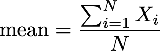
• The mean denotes the average of the group of finite numbers. The sample mean is approximately equal to the population mean.
  

• The standard deviation tells us how much the values in the sample/ population is spread out from the mean value.
  

• Variance gives us a measure of the degree to which each value in the population/sample differs from the mean value. It is expressed as the average of the squared differences of data points from the mean value or simply, the square of standard deviation.
  

Covariance and correlation

In statistics, Covariance is used to identify how they both change together and also the relationship between them. Usually, covariance is used to classify three types of relationships between two variables. They are:

• Relationship with positive trends (similar to direct proportionality)
• Relationship with negative trends (similar to inverse proportionality)
• Times when there is no relationship/trend

We can calculate covariance for the population using:

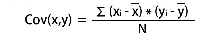
Correlation is dimensionless and is used to quantify the relationship between two variables. It has its range as [-1,1]. A negative correlation means that the variables share a weak relationship and the data with a strong relationship has a high correlation value.

where sigma represents the standard deviation of the respective variable.

Hypothesis Testing

Hypothesis testing helps us identify whether an action should be performed or not based on the results it will yield. In hypothesis testing, we usually consider two hypotheses: Null and alternative. The version of the outcome that has higher chance of failure is usually considered as null hypothesis and the alternate positive version is considered as the alternative hypothesis.

After this, a test statistic is calculated and one of the various statistical tests available: F-test, Chi square test, etc. is chosen.

The critical value depends on the significance level ( which is usually taken as 5%) and this value divides the curve into rejection and non-rejection region.

If the test statistic is more extreme than the critical value, the the null hypothesis is rejected. If not, it is not rejected.

Regression

Regression is a statistical method that help in finding out the relationship between independent and dependent variables and also model them out. If only one independent variable is present, then it is known as linear regression and if many are there, then it is multiple regression. Regression models form a major portion of Machine learning and are used widely.

Bayes theorem

Bayes theorem is one of the well-known theorems in the world of statistics and probability. It revolves around the concept of conditional probability. Conditional probability, in simple words, is the probability or chance of an event happening given that another related event had already occurred.

For example, suppose we have 1000 people who have a particular disease, out of which 400 are women. Now if we want to know the probability of a woman having this disease, then this comes under conditional probability. Here, the condition given to us is that the person must be a woman.

The formula is as follows:

where,

• Pr(X|Y) is the probability of event X occurring given event Y had occurred.
• Pr(X) and Pr(Y) are probabilities of events X and Y occurring respectively.
• Pr(Y|X) is the probability of event Y happening given that X had already happened.

Going along the lines of our example, Pr(X|Y) is the probability of a woman getting the disease, Pr(Y|X) is the probability of a person who already got the disease being a woman (2/5 from the above given numbers), Pr(X) and Pr(Y) are probabilities of getting the disease and probability of being a woman.

Distribution of data

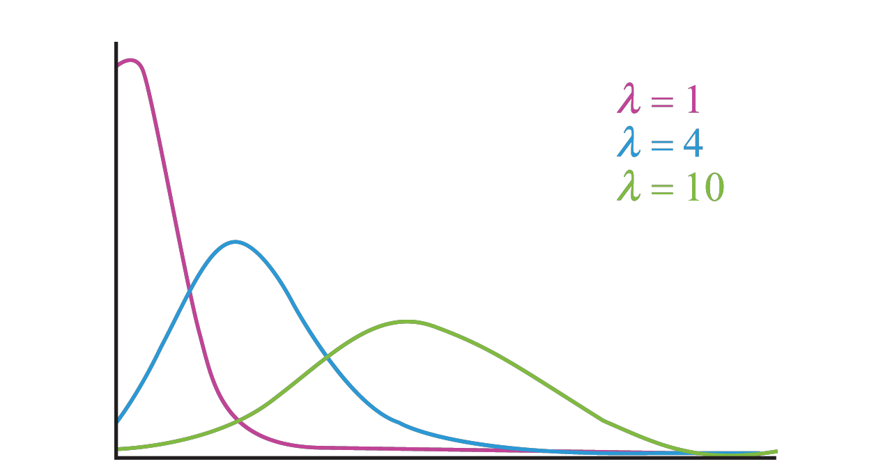
Identifying how data is distributed plays an important role to make judgements about the population. Distributions like the Normal distribution is very significant. And this goes along with laws like the Law of Large Numbers and Central limit theorem which tells us that the parameters generated and the statistical inferences become more accurate when more data is gathered. Given below are visualizations of some distributions in Probability.

• Poisson Distribution
  

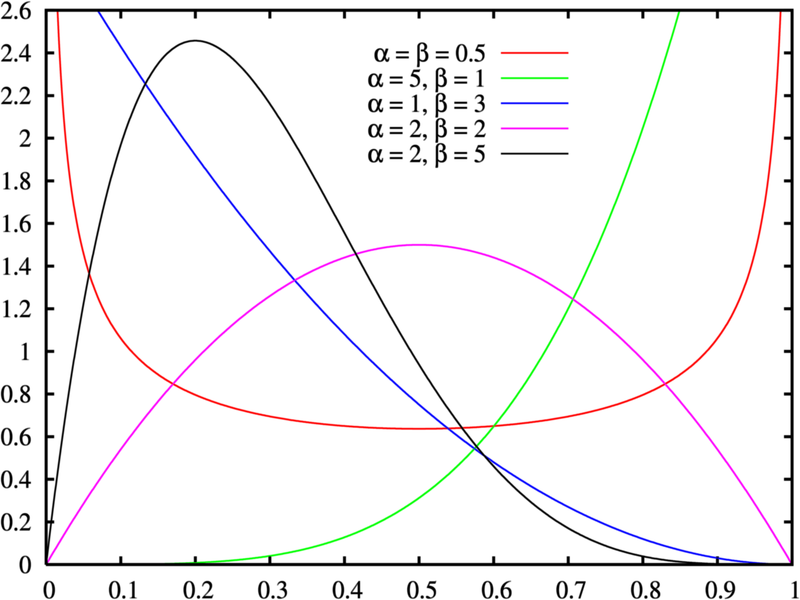
• Beta Distribution
  

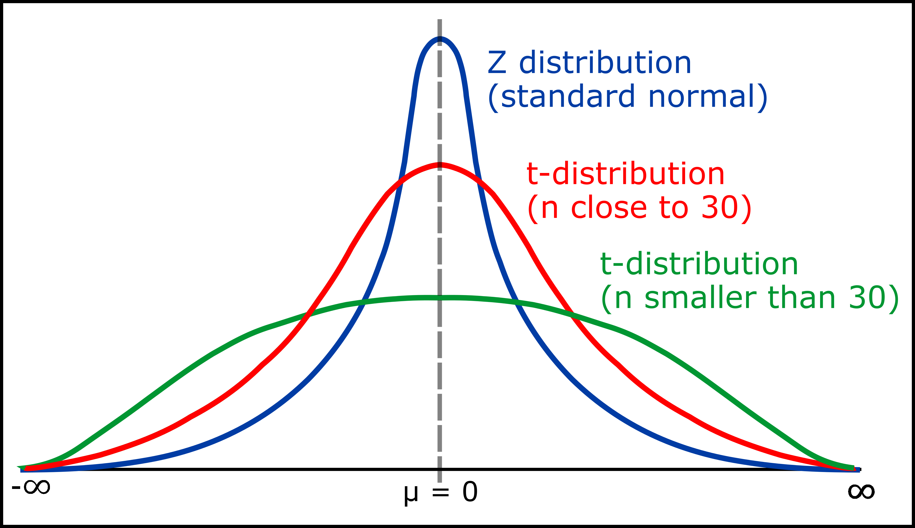
• Comparison between normal distribution and student's t distribution
  

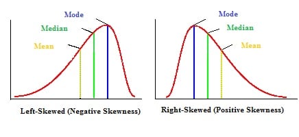
• Skewed distribution
  
  
  

Introduction to Linear algebra for Data Science

Linear algebra is a domain of mathematics that deals with linear equations. It can be as simple as the famous straight line equation ( y= mx + c) for two-dimension. But as the number of dimensions increases, it gets more complex.

Probability and Statistics were easier to relate to Data Science. But where is Linear algebra used in Data Science?

We know that the images bits are stored as their numerical equivalent. So the bits of a whole image would represent a matrix. In image convolution, the feature maps and filters also are in form of matrices. The Principle Component Analysis (PCA) is a technique that is used to reduce the dimensionality. Reducing the number of dimensions with as little data loss as possible is an important step in machine learning before processing the data. Eigenvectors are extensively used in PCA. The loss functions in linear algebra are extensively used in machine learning models to measure the accuracy of the model.

Now we know some uses of linear algebra in data science, let us take a look at some of these concepts.

Loss functions

While there are many loss functions in linear algebra, the ones that are commonly used are Mean Squared Error (MSE) and Mean Absolute Error (MAE).

Mean Squared Error

This is easier to understand and is the one that is mostly used in machine learning models. First, we calculate the difference between the observed and predicted value for all data points. Square the differences and add them all to obtain the cumulative squared error. Then divide it by the total number of data points to obtain the mean/average squared error. It can be represented as follows:

Mean Absolute Error

This is similar to MSE, but here, we take the absolute difference of the observed and predicted values.

However, implementing the modulus function in ML models can be difficult at times.

Matrix

A matrix is a 2-D array of numbers and is characterized by its rows and columns. A m x n matrix means a matrix that contains m rows and n columns. Given below is a 2x4 matrix.

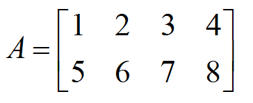
• In addition of two matrices A and B, we obtain the resultant matrix by just adding the elements in A with corresponding elements in B.
  

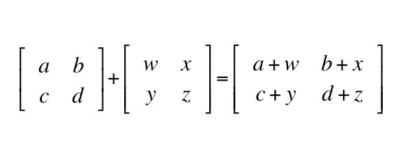
• In multiplication of a matrix with a scalar number, each element in the resultant matrix is a product of the scalar number and the corresponding element in the matrix.
  

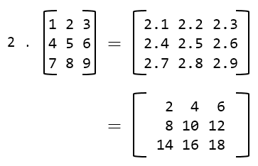
• Multiplication of two matrices is performed in a different way. Let A (m x n) and B (n x p) be the two matrices to be multiplied and C be the product matrix. The main condition to be satisfied is that the number of columns in A must be equal to the number of rows in B. C will be of order m x p. The element C_ij in the resultant matrix is the dot product of i^th row of A and j^th column of B.
  

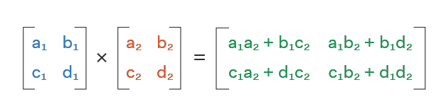
• Various equations can also be represented in matrix form, which makes them easier to solve using either Matrix Inverse or Manipulations.

Eigenvalues and Eigenvectors

When a matrix contains only one column, it is called a vector. In vectors, multiplying a vector with a matrix is called linear transformation. Eigenvector of a matrix is a vector whose direction remains the same even after applying linear transformation with the matrix. The eigenvalue is a scalar value which is associated with the linear transformation of the eigenvector. Both eigenvalues and vectors are applicable only if the matrix is a square matrix ( i.e. of order n x n).

Let A be the given square matrix. We find the eigenvalue (λ) by using the equation |A-λI|=0 where I is the identity matrix. Once we know the values of λ, we substitute it in the equation Av=λv where v is the eigenvector. We obtain the eigenvector by solving the different equations we get from substituting different λ values in the equation.

Let us understand this with an example. Let the given matrix be

To find the Eigenvalues and Eigenvectors, we use the characteristic equation

Solving the equation, we get the Eigenvalues to be λ1=-1, λ2=-2. Now we find the 2 Eigenvectors. The Eigenvector v₁ is associated with λ1=-1 and v₂ with λ2=-2.
Now let us find v₁

Performing matrix multiplication on the top row, we get

then from the second row we get

So, we conclude that the elements of v₁ are equal in magnitude and have opposite signs. Therefore,

where k₁ is an arbitrary constant. Here, we could have used any quantities equal in magnitude and havve opposite signs instead of -1 and +1.

Following the same procedure for v₂,

Here too the values +1 and -2 are arbitrary. Only the ratios of the values are important.


Another important domain of mathematics used in Data Science is Calculus. One of the popular example of Calculus in Data Science is the Gradient descent. Intimate knowledge of only statistics, probability and linear algebra are extensively needed in data science.

With this article at OpenGenus, you must have a strong hold on Mathematics for Data Science.