
This is the most complete Data Science Cheatsheet which you should follow to revise all Data Science concepts within 30 minutes and get ready for Interviews and stay in form.

| Data science lifecycle | ||
|---|---|---|
| Phase | Description | |
| Discovery | ||
| Understanding data | Involves describing what data is needed, how relevant are they and finally extracting the required data. | |
| Data preparation | ||
| Data analysis | ||
| Model planning | Decide on our machine learning model based on the business problem. | |
| Model building and deployment | Create and evaluate the ML model and finally deploy it in the preferred environment. | |
| Communication of results | ||
| Machine Learning | ||
|---|---|---|
| Supervised Learning | Type of machine learning technique where models are trained using labeled data as inputs. Commonly used fore regression and classification tasks. | |
| Unsupervised Learning | Type of machine learning technique where models are trained using unalbeled data as inputs. Used for extracting information from large amounts of data. | |
| Semi-supervised Learning | Combination of supervised and unsupervised learning where a small amount of inputs are labeled and large portions of them are unlabeled. | |
| Reinforcement Learning | This is a machine learning technique concerned with teaching agents to take decisions in environment to maximize the reward. | |
| Regression | ||
| Classification | These algorithms are used to categorize the given test data accurately, such as telling apart a cat from a dog. | |
| Ensemble Learning | Ensemble methods helps improve the performance of a machine learning model by combining several ML base models to produce one single predictive model. | |
| Recommender Systems | ||
| Supervised Learning | |||
|---|---|---|---|
| Algorithm | Description | Advantages | Disadvantages |
| Logistic Regression | An algorithm that models linear relationship between inputs and outputs a categorical variable. | ||
| Linear Regression | An algorithm that models linear relationship between inputs and produces continuous outputs. | ||
| Support Vector Machines | An algorithm that aims to create the best decision boundary to group n-dimensional space into different classes. | ||
| Random Forest | It is a combination of many decision trees and is an ensemble learning method. | ||
| Decision Tree | An algorithm that can be used for both regression and classification where models make decision rules on features to obtain predictions. | ||
| K-Nearest Neighbors | An algorithm that uses feature similarity to predict values of new data points. | ||
| Unsupervised Learning | |||
|---|---|---|---|
| Algorithm | Description | Advantages | Disadvantages |
| K-Means Clustering | A clustering algorithm that determines K clusters based on euclidean distances. | ||
| Hierarchical Clustering | |||
| DBSCAN | |||
| Apriori Algorithm | |||
| Principal Component Analysis | This algorithm is widely used for dimensionality reduction. | ||
| Manifold Learning | It is used for non-linear dimensionality reduction and aims to describe datasets as low-dimensional manifolds embedded in high-dimensional spaces. | ||
| Deep Learning | ||
|---|---|---|
| Neural Network | A neural network takes an input, passes it through multiple layers of hidden neurons and outputs a prediction representing the combined input of all the neurons. | |
| Architectures |
| |
| LSTM | LSTM is a variant of RNN that is used for learning long term dependencies. It has a memory cell to record additional information. | |
| Back propagation | A back propagation algorithm consists of two main steps:
| |
| Gradient descent | ||
| Activation function | ||
| Loss function | ||
| Optimizers | | |
| Regularization | It is a technique for combating overfitting and improving training. Some of them are early stopping, data augmentation and ensembling. | |
| Layers |
| |
| Python Basics | ||
|---|---|---|
| Concept | Code | Description |
| NumPy | ||
| Creating arrays | ||
| Inspecting the array | ||
| Arithmetic Operations | ||
| Aggregate functions | ||
| Subsetting and Slicing | ||
| Array manipulation | ||
| Pandas | ||
| Series | s = pd.Series([3, -5, 7, 4], index=['a', 'b', 'c', 'd']) | A one-dimensional labeled array a capable of holding any data type |
| DataFrame | data = {'Country': ['Belgium', 'India', 'Brazil'],
'Capital': ['Brussels', 'New Delhi', 'Brasília'],
'Population': [11190846, 1303171035, 207847528]} df = pd.DataFrame(data, columns=['Country', 'Capital', 'Population']) | A two-dimensional labeled data structure with columns of potentially different types |
| Reading csv files | pd.read_csv('file.csv', header=None, nrows=5) | |
| Selecting and setting | ||
| Sorting and dropping | ||
| Retrieving basic dataframe information | ||
| Summary of dataframe information | ||
| Statistics and Probability | ||
|---|---|---|
| Concept | Description | Formula/Graph |
| Mean | The mean denotes the average of the group of finite numbers. | 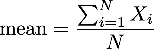 |
| Median | The median denotes the middle of an ordered set of data. | 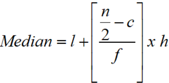 |
| Mode | Is only relevant for discrete data and is the the most common value occurring in a dataset. | 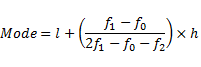 |
| Variance | Variance gives a measure of the degree to which each value in the population/sample differs from the mean value. | 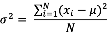 |
| Standard deviation | The standard deviation tells us how much the values in the sample/ population is spread out from the mean value. | 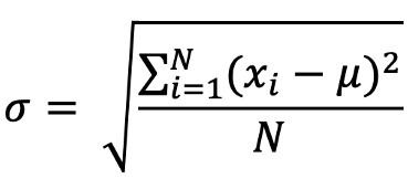 |
| Covariance | Covariance is used to identify how they both change together and also the relationship between them. | 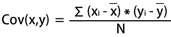 |
| Correlation | Correlation is dimensionless and is used to quantify the relationship between two variables. It has its range as [-1,1]. | 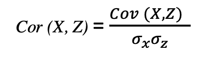 |
| Central limit theorem | It states that "As the sample size becomes larger, the distribution of sample means approximates to a normal distribution curve." | |
| Law of large numbers | The law of large numbers states that As the number of trials or observations increases, the actual or observed average approaches the theoretical or expected average. | |
| Bayes theorem | 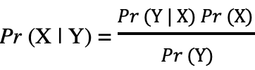 | |
| Hypothesis testing | ||
| A/B testing | A/B testing is a famous testing technique used to compare two variants to determine the best of the two based on user experience. | |
| Confidence intervals | A Confidence interval expresses a range of values within which we are pretty sure that the population parameter lies | 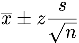 |
| Normal distribution | 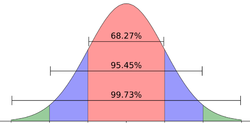 | |
| Poisson distribution | Distribution that expresses the probability of a given number of events occurring within a fixed time period | 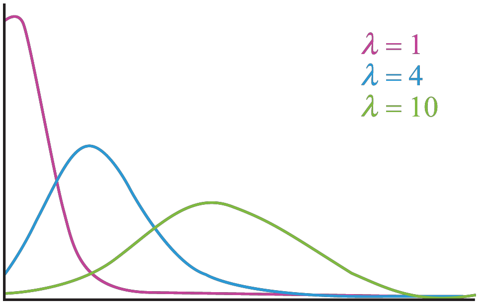 |
| Data visualization | ||
|---|---|---|
| Chart | Description | Image |
| Capturing trends | ||
| Line chart | 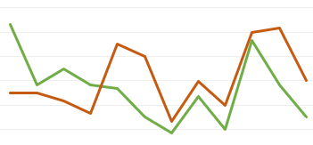 | |
| Area chart | 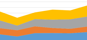 | |
| Capturing distributions | ||
| Histogram | 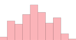 | |
| Boxplot | Shows the distribution of a variable using 5 key summary statistics. | 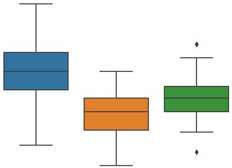 |
| Violinplot | 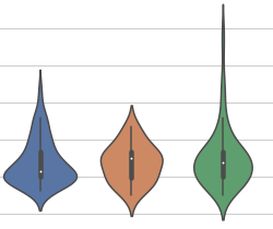 | |
| Part to-whole charts | ||
| Pie chart | 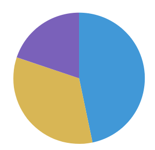 | |
| Donut chart | 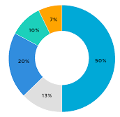 | |
| Heatmap | 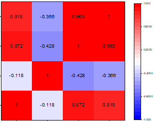 | |
| Stacked chart | Compare subcategories within categorical data. | 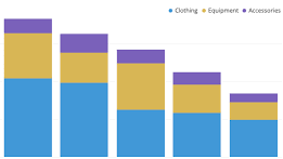 |
| Visualising relationships | ||
| Bar/column chart |  | |
| Scatter plot |  | |
| Bubble chart |  | |
| Time series analysis | ||
|---|---|---|
| Concept | Description | Code |
| ACF plot | The autocorrelation function (ACF) plot shows the autocorrelation coefficients as a function of the lag. | import statsmodels.api as sm sm.graphics.tsa.plot_acf(data) |
| PACF plot | The partial autocorrelation function (PACF) plot shows the partial autocorrelation coefficients as a function of the lag. | import statsmodels.api as sm sm.graphics.tsa.plot_pacf(data) |
| ADF test | If a series is stationary, its mean, variance, and autocorrelation are constant over time. We can test for stationarity with augmented Dickey-Fuller (ADF) test. | from statsmodels.tsa.stattools import adfuller p_value= adfuller(data) |
| Time series decomposition | Separate the series into 3 components: trend,seasonality, and residuals | from statsmodels.tsa.seasonal import STL decomp=STL(data,period=m).fit() plt.plot(decomp.observed) plt.plot(decomp.trend) plt.plot(decomp.seasonal) plt.plot(decomp.resid) |
| Moving average model – MA(q) | The moving average model: the current value depends on the mean of the series, the current error term, and past error terms. | from statsmodels.tsa.statespace.sarimax import SARIMAX model=SARIMAX(data,order=(0,0,q)) |
| Autoregressive model – AR(p) | The autoregressive model is a regression against itself. This means that the present value depends on past values.
| from statsmodels.tsa.statespace.sarimax import SARIMAX model=SARIMAX(data,order=(p,0,0)) |
| ARMA(p,q) | The autoregressive moving average model (ARMA) is the combination of the autoregressive model AR(p), and the moving average model MA(q). | from statsmodels.tsa.statespace.sarimax import SARIMAX model=SARIMAX(data,order=(p,0,q)) |
| ARIMA(p,d,q) | The autoregressive integrated moving average (ARIMA) model is the combination of the autoregressive model AR(p), and the moving average model MA(q), but in terms of the differenced series. | from statsmodels.tsa.statespace.sarimax import SARIMAX model=SARIMAX(data,order=(p,d,q)) |
| SARIMA(p,d,q)(P,D,Q)m | The seasonal autoregressive integrated moving average (SARIMA) model includes a seasonal component on top of the ARIMA model. | from statsmodels.tsa.statespace.sarimax import SARIMAX model=SARIMAX(data,order=(p,d,q),seasonal_order=(P,D,Q,m)) |