Hyperplane in SVM

Introduction

Support Vector Machines (SVMs) are powerful machine learning models that can be used for both classification and regression tasks. In classification, the goal is to find a hyperplane that separates the data points of different classes with maximum margin. This hyperplane is known as the "optimal hyperplane" or "maximum-margin hyperplane".

To understand the concept of the hyperplane in SVMs, let's dive deeper into the working of SVMs and how the optimal hyperplane is determined

Support Vector Machines

Support Vector Machines (SVMs) are supervised learning models that analyze and classify data. SVMs find an optimal hyperplane that best separates the data points of different classes. The hyperplane serves as the decision boundary, enabling SVMs to make predictions on unseen data.

The main idea behind SVMs is to find a hyperplane or decision boundary that maximizes the margin between the support vectors of different classes. Support vectors being the data points closest to the decision boundary. This article goes into more depth on SMVs:https://iq.opengenus.org/understand-support-vector-machine-in-depth/

Hyperplane

In SVMs, a hyperplane is a subspace of one dimension less than the original feature space. In two-dimensional space, a hyperplane is a line, while in three-dimensional space, it is a plane. In general, in n-dimensional space, a hyperplane is an (n-1)-dimensional flat affine subspace.

The hyperplane in SVMs is represented by the equation:

where w is the weight vector, x is a data point, and b is the bias term. The weight vector determines the "shape" of the hyperplane, and the bias term determines the position of it.

The decision rule for SVMs is based on the sign of the equation above. If the result is positive, the data point is classified as one class, and if it is negative, the data point is classified as the other class.

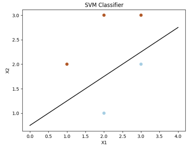
Here we can see an example where the data is in two dimenssions and the hyperplane is a 1-d line.

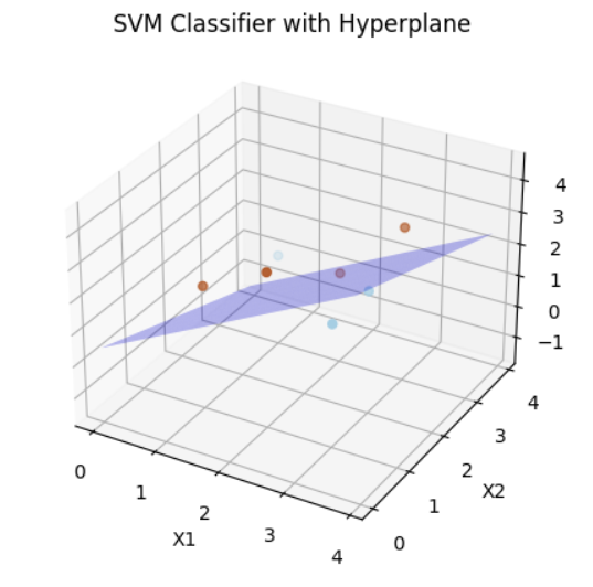
Here the data has 3 dimensions and the classes are seperated by a 2d hyperplane.

Finding the best hyperplane

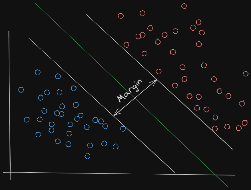
The data points that lie closest to the hyperplane/the decision boundary are called support vectors. These support vectors play a crucial role in determining the optimal hyperplane. The distance between the hyperplane and the support vectors is known as the margin. The SVM tries to maximize this margin, as it provides a measure of the confidence of classification. In a sense the longer the distance between the different classes the more clearly they are separated which indicates a higher confidence level of classification.

Question: So what does that mean for any points on the hyperplane?
These points are in the middle of the 2 classes, which can be interpreted as we don't know what class that they belong to.

Therefore we can reason that the optimal hyperplane is the one that maximizes the margin between the two classes.

The margin is defined as the perpendicular distance between the hyperplane and the closest data points from each class. These closest data points are called support vectors.

Let's denote the support vectors as x_+ for class 1 and x_- for class -1. The distance between these support vectors is given by:

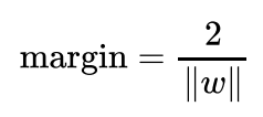
Where ||w|| represents the Euclidean norm of the weight vector w. The goal of SVM is to find the hyperplane that maximizes this margin, which in turn improves the generalization performance of the classifier.

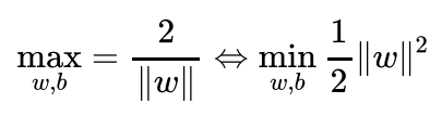
To find the optimal hyperplane, SVM solves either the following maximization or the equivalent minimization -problem an optimization problem:

subject to the constraints:

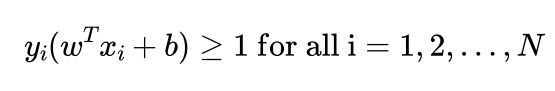
Here, N represents the number of data points, and y_i represents the class labels. The constraints ensure that all data points are correctly classified and lie on the correct side of the margin.

The optimization problem can be solved using various algorithms, such as the Sequential Minimal Optimization (SMO) or the Interior Point Methods. Once the optimization problem is solved, the learned parameters w and b define the optimal hyperplane that separates the two classes with the maximum margin.

Implementation

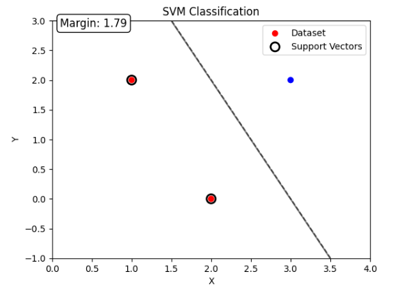
using the above equations and applying it in python (the minimization problem is solved using the function minimize from the package scipy.optimize):

import numpy as np
import matplotlib.pyplot as plt

# Step 1: Define the dataset
X = np.array([[1, 2], [2, 0], [3, 2]])  # Features
y = np.array([1, 1, -1])  # Labels

# Step 2: Define the SVM optimization problem
def objective(w):
    return 0.5 * np.linalg.norm(w)**2

def constraint(w):
    return y * (np.dot(X, w[:-1]) + w[-1]) - 1

# Step 3: Solve the SVM optimization problem
initial_guess = np.zeros(X.shape[1] + 1)  # Initial guess for w and b
bounds = [(None, None)] * X.shape[1] + [(None, None)]  # No bounds on w and b

from scipy.optimize import minimize

solution = minimize(objective, initial_guess, bounds=bounds, constraints={'type': 'ineq', 'fun': constraint})

# Step 4: Extract the optimal parameters
w = solution.x[:-1]
b = solution.x[-1]

# Calculate the margin
margin = 2 / np.linalg.norm(w)

# Plotting the results
plt.scatter(X[:, 0], X[:, 1], c=y, cmap='bwr', label='Dataset')

# Plotting the decision boundary
x_min, x_max = X[:, 0].min() - 1, X[:, 0].max() + 1
y_min, y_max = X[:, 1].min() - 1, X[:, 1].max() + 1
xx, yy = np.meshgrid(np.arange(x_min, x_max, 0.01), np.arange(y_min, y_max, 0.01))
grid_points = np.c_[xx.ravel(), yy.ravel()]
decision_values = np.dot(grid_points, w) + b
Z = np.sign(decision_values).reshape(xx.shape)
plt.contour(xx, yy, Z, colors='k', levels=[-1, 0, 1], alpha=0.5)

# Plotting the margin
support_vectors = X[solution.success]
plt.scatter(support_vectors[:, 0], support_vectors[:, 1], s=100, facecolors='none', edgecolors='k', linewidths=2, label='Support Vectors')

# Setting plot limits and labels
plt.xlim(x_min, x_max)
plt.ylim(y_min, y_max)
plt.xlabel('X')
plt.ylabel('Y')
plt.title('SVM Classification')
plt.legend()

# Display the margin
plt.text(x_min + 0.1, y_max - 0.1, f'Margin: {margin:.2f}', fontsize=12, bbox=dict(facecolor='white', edgecolor='black', boxstyle='round'))

plt.show()

comparing to the sklearn svm function:

from sklearn.svm import SVC

# Step 1: Define the dataset
X = [[1, 2], [2, 0], [3, 2]]  # Features
y = [1, 1, -1]  # Labels

# Step 2: Create and fit the SVM classifier
clf = SVC(kernel='linear')
clf.fit(X, y)

# Step 3: Calculate the weight vector, bias term, and margin
w = clf.coef_[0]
b = clf.intercept_[0]
margin = 2 / np.linalg.norm(w)

# Step 4: Print the results
print("Weight Vector:", w)
print("Bias Term:", b)
print("Margin:", margin)

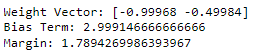
The results looks similar indicating that our formulas are working.

Conclusion

In conclusion, Support Vector Machines (SVMs) are powerful machine learning models used for classification and regression tasks. SVMs find an optimal hyperplane that separates data points of different classes with maximum margin. The hyperplane serves as the decision boundary, enabling SVMs to make predictions on unseen data.

The key concepts in SVMs discussed in this article includes the hyperplane, which is the subspace that separates data points, and support vectors, which are the data points closest to the hyperplane.

The goal of SVMs is to find the hyperplane that maximizes the margin between the support vectors of different classes. As this margin represents the confidence of classification so a larger margin means a higher confidence of the classification.