Bin Packing problem involves assigning n items of different weights and bins each of capacity c to a bin such that number of total used bins is minimized. It may be assumed that all items have weights smaller than bin capacity.

Table of contents:

1. Mathematical Formulation of Bin Packing
2. A brief outline of Approximate Algorithms
3. Lower Bound on Bins
4. Input Order dependent or Online Algorithms
   • Next Fit algorithm
   • First Fit algorithm
   • Best Fit Algorithm
   • Worst Fit Algorithm
5. Input Order Independent or Offline Algorithms
   • First Fit Decreasing
   • Best Fit Decreasing
6. Applications of Bin-Packing Algorithms

If you like to learn more about Approximate Algorithms, go through these articles:

• Introduction to Approximation Algorithms
• Approximate algorithms for NP problems
• Probabilistic / Approximate Counting
• Approximation Algorithm for Travelling Salesman Problem

Let us get started with Bin Packing problem.

Mathematical Formulation of Bin Packing

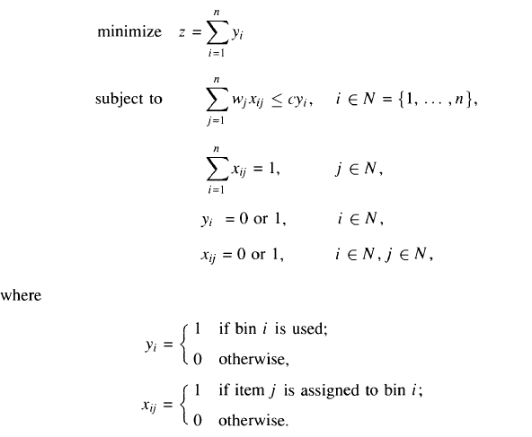
The Bin-Packing Problem (BPP) can also be described,using the terminology of
knapsack problems, as follows. Given n items and n knapsacks (or bins), with

Wj = weight of item j,
cj = capacity of each bin

assign each item to one bin so that the total weight of the items in each bin does
not exceed c and the number of bins used is a minimum. A possible mathematical
formulation of the problem is

We will suppose, as is usual, that the weights Wj are positive integers. Hence,
without loss of generality, we will also assume that c is a positive integer

Wj < c for j belonging to N.

As you can see, we have a broad rule of approximation and not an exact algorithm. Such algorithms are called NP problems. In fact Bin Packing Problem is a NP-hard problem

A brief outline of Approximate Algorithms

Many optimization problems exist for which there is no known polynomial time algorithm for its execution.

Approximation algorithms allow for getting a solution close to the (optimal) solution of an optimization problem in polynomial time.

An algorithm is an α-approximation algorithm for an optimized problem if:

• The algorithm runs in polynomial time
• The algorithm always produces a solution that is within a factor of α of the optimal solution

For a given problem instance I,

Approximation ratio(α) = Algo(I)/z(I),

where Algo(I) is the algorithm under scrutiny and z(I) is the optimal solution.
For the Bin-Packing problem, let us consider bins of size 1

Assuming the sizes of the items be {0.5, 0.7, 0.5, 0.2, 0.4, 0.2, 0.5, 0.1, 0.6}.
The most optimal solution (z(I))for this instance I would be

Lower Bound on Bins

We can always find a lower bound on minimum number of bins required. The lower bound can be given as :

Min no. of bins  >=  Ceil ((Total Weight) / (Bin Capacity))

Let us now look at the various optimization algorithms for Bin Packing Problem.

Input Order dependent or Online Algorithms

The following 4 algorithms depend on the order of their inputs. They pack the item given first and then move on to the next input or next item

1) Next Fit algorithm

The simplest approximate approach to the bin packing problem is the Next-Fit (NF) algorithm which is explained later in this article. The first item is assigned to bin 1. Items 2,... ,n are then considered by increasing indices : each item is assigned to the current bin, if it fits; otherwise, it is assigned to a new bin, which becomes the current one.

Visual Representation

Let us consider the same example as used above and bins of size 1

Assuming the sizes of the items be {0.5, 0.7, 0.5, 0.2, 0.4, 0.2, 0.5, 0.1, 0.6}.

The minimum number of bins required would be Ceil ((Total Weight) / (Bin Capacity))=
Celi(3.7/1) = 4 bins.

The Next fit solution (NF(I))for this instance I would be-

Considering 0.5 sized item first, we can place it in the first bin

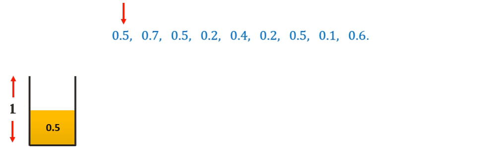
Moving on to the 0.7 sized item, we cannot place it in the first bin. Hence we place it in a new bin.

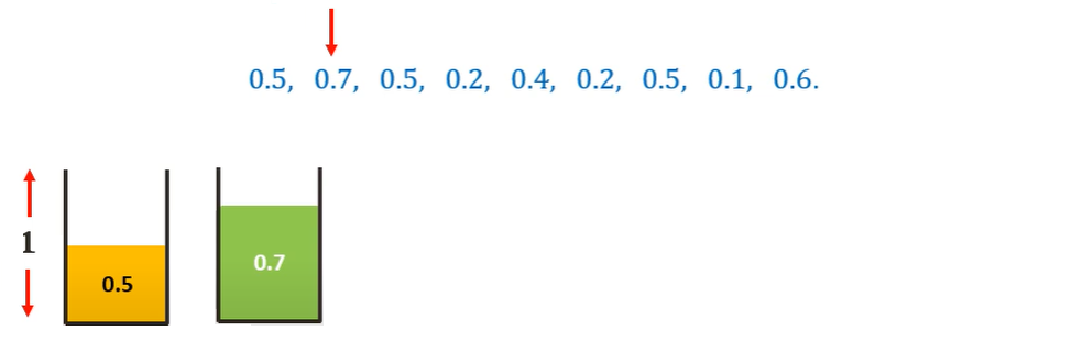
Moving on to the 0.5 sized item, we cannot place it in the current bin. Hence we place it in a new bin.

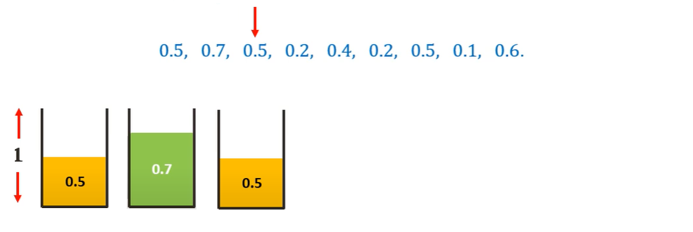
Moving on to the 0.2 sized item, we can place it in the current (third bin)

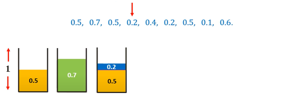
Similarly, placing all the other items following the Next-Fit algorithm we get-

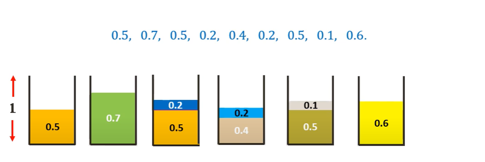
Thus we need 6 bins as opposed to the 4 bins of the optimal solution. Thus we can see that this algorithm is not very efficient.

Analyzing the approximation ratio of Next-Fit algorithm

The time complexity of the algorithm is clearly O(n). It is easy to prove that, for any instance I of BPP,the solution value NF(I) provided by the algorithm satisfies the bound

NF(I)<2z(I)

where z(I) denotes the optimal solution value. Furthermore, there exist instances for which the ratio NF(I)/z(I) is arbitrarily close to 2, i.e. the worst-case approximation ratio of NF is r(NF) = 2.

Psuedocode

NEXT FIT (size[], n, c)

size[] is the array containg the sizes of the items, n is   the number of items and c is the capacity of the bin

{

    Initialize result (Count of bins) and remaining capacity in current bin.
    res = 0
    bin_rem = c
 
    Place items one by one
    for (int i = 0; i < n; i++) {
        // If this item can't fit in current bin
        if (size[i] > bin_rem) {
            Use a new bin
            res++ 
            bin_rem = c - size[i]
        }
        else
            bin_rem -= size[i];
    }
    return res;
}

Let us look at the implementation of the program in C++

#include <bits/stdc++.h>
using namespace std;

int nextFit(double size[], int n, int c)
{
    
    int res = 0, bin_rem = c;
    
    for (int i = 0; i < n; i++) {        
        if (size[i] > bin_rem) {
            res++; 
            bin_rem = c - size[i];
        }
        else
            bin_rem -= size[i];
    }
    return res;
}
 

int main()
{
    double size[] = {0.5, 0.7, 0.5, 0.2, 0.4, 0.2, 0.5, 0.1, 0.6};
    int c = 1;
    int n = sizeof(size) / sizeof(size[0]);
    cout << "Number of bins required in Next Fit : "<< nextFit(size, n, c);
    return 0;
}

Output: Number of bins required in Next Fit : 6

Complexity

• Worst case time complexity: Θ(n)
• Average case time complexity: Θ(n)
• Best case time complexity: Θ(n)
• Space complexity: Θ(n)

2) First Fit algorithm

A better algorithm, First-Fit (FF), considers the items according to increasing
indices and assigns each item to the lowest indexed initialized bin into which it
fits; only when the current item cannot fit into any initialized bin, is a new bin
introduced

Visual Representation

Let us consider the same example as used above and bins of size 1

Assuming the sizes of the items be {0.5, 0.7, 0.5, 0.2, 0.4, 0.2, 0.5, 0.1, 0.6}.

The minimum number of bins required would be Ceil ((Total Weight) / (Bin Capacity))=
Celi(3.7/1) = 4 bins.

The First fit solution (FF(I))for this instance I would be-

Considering 0.5 sized item first, we can place it in the first bin

Moving on to the 0.7 sized item, we cannot place it in the first bin. Hence we place it in a new bin.

Moving on to the 0.5 sized item, we can place it in the first bin.

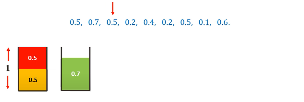
Moving on to the 0.2 sized item, we can place it in the first bin, we check with the second bin and we can place it there.

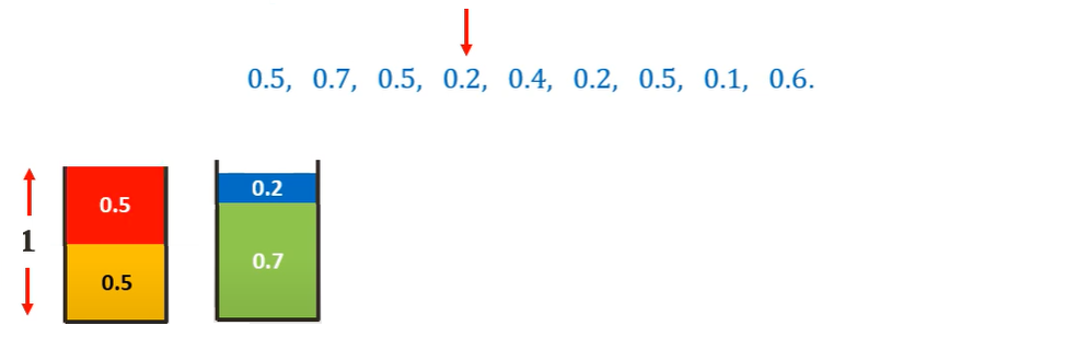
Moving on to the 0.4 sized item, we cannot place it in any existing bin. Hence we place it in a new bin.

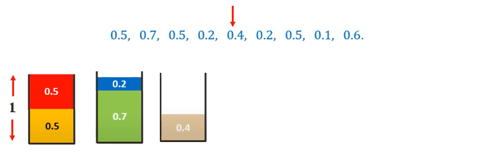
Similarly, placing all the other items following the First-Fit algorithm we get-

Thus we need 5 bins as opposed to the 4 bins of the optimal solution but is much more efficient than Next-Fit algorithm.

Analyzing the approximation ratio of Next-Fit algorithm

If FF(I) is the First-fit implementation for I instance and z(I) is the most optimal solution, then:

It can be seen that the First Fit never uses more than 1.7 * z(I) bins. So First-Fit is better than Next Fit in terms of upper bound on number of bins.

Psuedocode

FIRSTFIT(size[], n, c)
{
size[] is the array containg the sizes of the items, n is   the number of items and c is the capacity of the bin


    /Initialize result (Count of bins)
    res = 0;
 
    Create an array to store remaining space in bins there can be at most n bins
    bin_rem[n];
 
    Place items one by one
    for (int i = 0; i < n; i++) {
        Find the first bin that can accommodate weight[i]
        int j;
        for (j = 0; j < res; j++) {
            if (bin_rem[j] >= size[i]) {
                bin_rem[j] = bin_rem[j] - size[i];               
                break;
            }
        }
 
        If no bin could accommodate size[i]
        if (j == res) {
            bin_rem[res] = c - size[i];
            res++;
        }
       
    }
    return res;
}

Let us look at the implementation of the program in C++

#include <bits/stdc++.h>
using namespace std;

int firstFit(double size[], int n, int c)
{
    
    int res = 0;
    int bin_rem[n];
    for (int i = 0; i < n; i++) {        
        int j;
        for (j = 0; j < res; j++) {
            if (bin_rem[j] >= size[i]) {
                bin_rem[j] = bin_rem[j] - size[i];               
                break;
            }
        }
 
        if (j == res) {
            bin_rem[res] = c - size[i];
            res++;
        }
       
    }
    return res;
}

int main()
{
    double size[] = {0.5, 0.7, 0.5, 0.2, 0.4, 0.2, 0.5, 0.1, 0.6};
    int c = 1;
    int n = sizeof(size) / sizeof(size[0]);
    cout << "Number of bins required in First Fit : "<< nextFit(size, n, c);
    return 0;
}

Output: Number of bins required in First Fit : 5

Complexity

• Worst case time complexity: Θ(n*n)
• Average case time complexity: Θ(n*n)
• Best case time complexity (Can be achieved using Self-balancing Binary trees): Θ(nlogn)
• Space complexity: Θ(n)

3) Best Fit Algorithm

The next algorithm, Best-Fit (BF), is obtained from FF by assigning the current
item to the feasible bin (if any) having the smallest residual capacity (breaking
ties in favor of the lowest indexed bin).

Simply put,the idea is to places the next item in the tightest spot. That is, put it in the bin so that the smallest empty space is left.

Visual Representation

Let us consider the same example as used above and bins of size 1

Assuming the sizes of the items be {0.5, 0.7, 0.5, 0.2, 0.4, 0.2, 0.5, 0.1, 0.6}.

The minimum number of bins required would be Ceil ((Total Weight) / (Bin Capacity))=
Celi(3.7/1) = 4 bins.

The First fit solution (FF(I))for this instance I would be-

Considering 0.5 sized item first, we can place it in the first bin

Moving on to the 0.7 sized item, we cannot place it in the first bin. Hence we place it in a new bin.

Moving on to the 0.5 sized item, we can place it in the first bin tightly.

Moving on to the 0.2 sized item, we cannot place it in the first bin but we can place it in second bin tightly.

Moving on to the 0.4 sized item, we cannot place it in any existing bin. Hence we place it in a new bin.

Similarly, placing all the other items following the First-Fit algorithm we get-

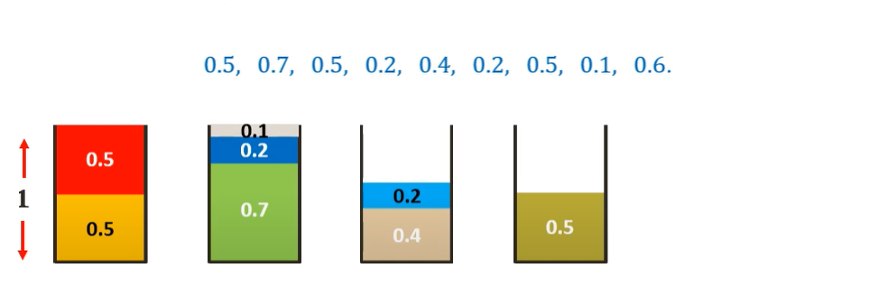
Thus we need 5 bins as opposed to the 4 bins of the optimal solution but is much more efficient than Next-Fit algorithm.

Analyzing the approximation ratio of Best-Fit algorithm

It can be noted that Best-Fit (BF), is obtained from FF by assigning the current item to the feasible bin (if any) having the smallest residual capacity (breaking ties in favour of the lowest indexed bin). BF satisfies the same worst-case bounds as FF

Analysis Of upper-bound of Best-Fit algorithm

If z(I) is the optimal number of bins, then Best Fit never uses more than 2 * z(I)-2 bins. So Best Fit is same as Next Fit in terms of upper bound on number of bins.

Psuedocode

BESTFIT(size[],n,  c)
{
size[] is the array containg the sizes of the items, n is   the number of items and c is the capacity of the bin
    Initialize result (Count of bins)
    res = 0;
 
    Create an array to store remaining space in bins there can be at most n bins
    bin_rem[n];
 
    Place items one by one
    for (int i = 0; i < n; i++) {
       
        Find the best bin that can accommodate weight[i]
        
        int j;
 
        Initialize minimum space left and index of best bin
        int min = c + 1, bi = 0;
 
        for (j = 0; j < res; j++) {
            if (bin_rem[j] >= size[i] && bin_rem[j] - size[i] < min) {
                bi = j;
                min = bin_rem[j] - size[i];
            }
        }
 
        If no bin could accommodate weight[i],create a new bin
        if (min == c + 1) {
            bin_rem[res] = c - size[i];
            res++;
        }
        else 
            Assign the item to best bin
            bin_rem[bi] -= size[i];
    }
    return res;
}

Let us look at the implementation of the program in C++

#include <bits/stdc++.h>
using namespace std;

int bestFit(double size[], int n, int c)
{
   
    int res = 0;
    int bin_rem[n];
    
    for (int i = 0; i < n; i++) {
        int j;
        int min = c + 1, bi = 0;
 
        for (j = 0; j < res; j++) {
            if (bin_rem[j] >= size[i] && bin_rem[j] - size[i] < min) {
                bi = j;
                min = bin_rem[j] - size[i];
            }
        } 
        
        if (min == c + 1) {
            bin_rem[res] = c - size[i];
            res++;
        }
        else 
            bin_rem[bi] -= size[i];
    }
    return res;
}
 

int main()
{
    double size[] = {0.5, 0.7, 0.5, 0.2, 0.4, 0.2, 0.5, 0.1, 0.6};
    int c = 1;
    int n = sizeof(size) / sizeof(size[0]);
    cout << "Number of bins required in Best Fit : "<< bestFit(size, n, c);
    return 0;
}

Output: Number of bins required in Best Fit : 5

Complexity

• Worst case time complexity: Θ(n*n)
• Average case time complexity: Θ(n*n)
• Best case time complexity (Can be achieved using Self-balancing Binary trees): Θ(nlogn)
• Space complexity: Θ(n)

4) Worst Fit Algorithm

This algorithm involves an idea to places the next item in the least tight spot to even out the bins. In other words, put it in the bin so that most empty space is left.

Analysis Of upper-bound of Worst-Fit algorithm

Worst Fit can also be implemented in O(n Log n) time using Self-Balancing Binary Search Trees.

If z(I) is the optimal number of bins , then Worst Fit never uses more than 2 * z(I)-2 bins. So Worst Fit is same as Next Fit in terms of upper bound on number of bins.

Psuedocode

WORSTFIT(size[], n, c)
{
size[] is the array containg the sizes of the items, n is   the number of items and c is the capacity of the bin

    Initialize result (Count of bins)
    res = 0;
 
    Create an array to store remaining space in bins there can be at most n bins
    bin_rem[n];
 
    Place items one by one
    for (int i = 0; i < n; i++) {
        Find the best bin that can accommodate size[i]
        j;
 
        Initialize maximum space left and index of worst bin
        mx = -1, wi = 0;
 
        for (j = 0; j < res; j++) {
            if (bin_rem[j] >= size[i] && bin_rem[j] - size[i] > mx) {
                wi = j;
                mx = bin_rem[j] - size[i];
            }
        }
 
        If no bin could accommodate size[i], create a new bin
        
        if (mx == -1) {
            bin_rem[res] = c - size[i];
            res++;
        }
        else 
            Assign the item to best bin
            bin_rem[wi] -= size[i];
    }
    return res;
}

Let us look at the implementation of the program in C++

#include <bits/stdc++.h>
using namespace std;

int worstFit(double weight[], int n, int c)
{
    
    int res = 0;
    int bin_rem[n];
 
    for (int i = 0; i < n; i++) {        
        int j;
        int mx = -1, wi = 0;
 
        for (j = 0; j < res; j++) {
            if (bin_rem[j] >= weight[i] && bin_rem[j] - weight[i] > mx) {
                wi = j;
                mx = bin_rem[j] - weight[i];
            }
        }
 
        
        if (mx == -1) {
            bin_rem[res] = c - weight[i];
            res++;
        }
        else 
            bin_rem[wi] -= weight[i];
    }
    return res;
}
 

int main()
{
    double weight[] = {0.5, 0.7, 0.5, 0.2, 0.4, 0.2, 0.5, 0.1, 0.6};
    int c = 1;
    int n = sizeof(weight) / sizeof(weight[0]);
    cout << "Number of bins required in Worst Fit : "<< bestFit(weight, n, c);
    return 0;
}

Output: Number of bins required in Worst Fit : 9

Explanation
To get the least 'tight' space or most free space, we can place each weight in a new bin. Since there are 9 items, we can place each item in a new bin. Therefore, Worst-fit, as the name suggests, is the worst of all algorithms when it comes to the large difference between the bins required and the optimal number of bins

Complexity

• Worst case time complexity: Θ(n*n)
• Average case time complexity: Θ(n*n)
• Best case time complexity (Can be achieved using Self-balancing Binary trees): Θ(nlogn)
• Space complexity: Θ(n)

Input Order Independent or Offline Algorithms

In the offline version, we have all items at our disposal since the start of the execution. The natural solution is to sort the array from largest to smallest, and then apply the algorithms discussed henceforth.

NOTE: In the online programs we have given the inputs upfront for simplicity but it can also work interactively

Let us look at the various offline algorithms

1) First Fit Decreasing

We first sort the array of items in decreasing size by weight and apply first-fit algorithm as discussed above

Algorithm

• Read the inputs of items
• Sort the array of items in decreasing order by their sizes
• Apply First-Fit algorithm

Visual Representation

Let us consider the same example as used above and bins of size 1

Assuming the sizes of the items be {0.5, 0.7, 0.5, 0.2, 0.4, 0.2, 0.5, 0.1, 0.6}.

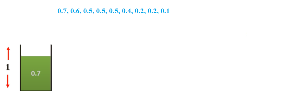
Sorting them we get {0.7, 0.6, 0.5, 0.5, 0.5, 0.4, 0.2, 0.2, 0.1}

The First fit Decreasing solution would be-

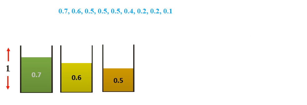
We will start with 0.7 and place it in the first bin

We then select 0.6 sized item. We cannot place it in bin 1. So, we place it in bin 2

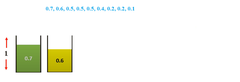
We then select 0.5 sized item. We cannot place it in any existing. So, we place it in bin 3

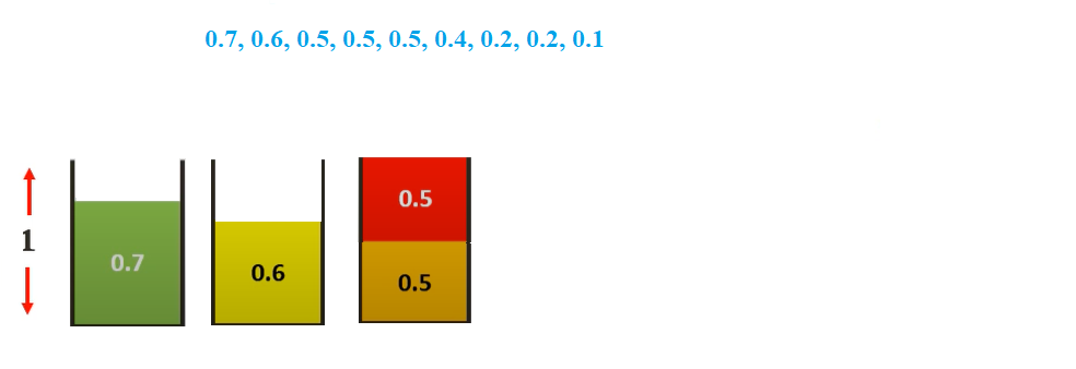
We then select 0.5 sized item. We can place it in bin 3

Doing the same for all items, we get.

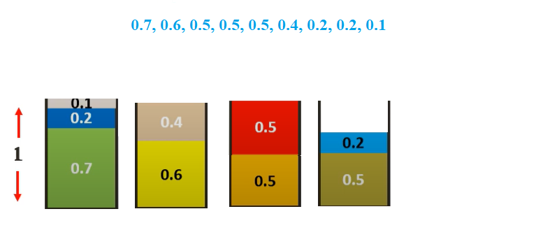
Thus only 4 bins are required which is the same as the optimal solution.

C++ Implementation

#include <bits/stdc++.h>
using namespace std;

void swap(double *xp, double *yp)
{
    double temp = *xp;
    *xp = *yp;
    *yp = temp;
}

int firstFit(double size[], int n, int c)
{
    
    int res = 0;
    int bin_rem[n];
    for (int i = 0; i < n; i++) {        
        int j;
        for (j = 0; j < res; j++) {
            if (bin_rem[j] >= size[i]) {
                bin_rem[j] = bin_rem[j] - size[i];               
                break;
            }
        }
 
        if (j == res) {
            bin_rem[res] = c - size[i];
            res++;
        }
       
    }
    return res;
}

int main()
{
    double size[] = {0.5, 0.7, 0.5, 0.2, 0.4, 0.2, 0.5, 0.1, 0.6};
    int c = 1;
    int n = sizeof(size) / sizeof(size[0]);
    
  
    for (int i = 0; i < n-1; i++) 
        for (int j = 0; j < n-i-1; j++)
            if (size[j] > size[j+1])
                swap(&size[j], &size[j+1]);
            
    cout << "Number of bins required in First Fit Decreasing : "<< nextFit(size, n, c);
    return 0;
}

Output: Number of bins required in First Fit Decreasing : 4

Complexity

• Worst case time complexity: Θ(n*n)
• Average case time complexity: Θ(n*n)
• Best case time complexity (Can be achieved using Self-balancing Binary trees): Θ(nlogn)
• Space complexity: Θ(n)

2) Best Fit Decreasing

We first sort the array of items in decreasing size by weight and apply Best-fit algorithm as discussed above

Algorithm

• Read the inputs of items
• Sort the array of items in decreasing order by their sizes
• Apply Next-Fit algorithm

Visual Representation

Let us consider the same example as used above and bins of size 1

Assuming the sizes of the items be {0.5, 0.7, 0.5, 0.2, 0.4, 0.2, 0.5, 0.1, 0.6}.
Sorting them we get {0.7, 0.6, 0.5, 0.5, 0.5, 0.4, 0.2, 0.2, 0.1}

The Best fit Decreasing solution would be-

We will start with 0.7 and place it in the first bin

We then select 0.6 sized item. We cannot place it in bin 1. So, we place it in bin 2

We then select 0.5 sized item. We cannot place it in any existing. So, we place it in bin 3

We then select 0.5 sized item. We can place it in bin 3

Doing the same for all items, we get.

Thus only 4 bins are required which is the same as the optimal solution.

C++ Implementation

#include <bits/stdc++.h>
using namespace std;

void swap(double *xp, double *yp)
{
    double temp = *xp;
    *xp = *yp;
    *yp = temp;
}

int bestFit(double size[], int n, int c)
{
   
    int res = 0;
    int bin_rem[n];
    
    for (int i = 0; i < n; i++) {
        int j;
        int min = c + 1, bi = 0;
 
        for (j = 0; j < res; j++) {
            if (bin_rem[j] >= size[i] && bin_rem[j] - size[i] < min) {
                bi = j;
                min = bin_rem[j] - size[i];
            }
        } 
        
        if (min == c + 1) {
            bin_rem[res] = c - size[i];
            res++;
        }
        else 
            bin_rem[bi] -= size[i];
    }
    return res;
}
int main()
{
    double size[] = {0.5, 0.7, 0.5, 0.2, 0.4, 0.2, 0.5, 0.1, 0.6};
    int c = 1;
    int n = sizeof(size) / sizeof(size[0]);
    
  
    for (int i = 0; i < n-1; i++) 
        for (int j = 0; j < n-i-1; j++)
            if (size[j] > size[j+1])
                swap(&size[j], &size[j+1]);
            
    cout << "Number of bins required in Best Fit Decreasing: "<< bestFirst(size, n, c);
    return 0;
}

Output: Number of bins required in Best Fit Decreasing : 4

Complexity

• Worst case time complexity: Θ(n*n)
• Average case time complexity: Θ(n*n)
• Best case time complexity (Can be achieved using Self-balancing Binary trees): Θ(nlogn)
• Space complexity: Θ(n)

Applications of Bin-Packing Algorithms

• Loading of containers like trucks.
• Placing data on multiple disks.
• This is used extensively while transporting goods over ships
• Job scheduling.

With this article at OpenGenus, you must have a strong idea of solving Bin Packing Problem efficiently.