
Get this book -> Problems on Array: For Interviews and Competitive Programming
Reading time: 20 minutes | Coding time: 5 minutes
If you are unfamiliar with the clustering problem, it is advisable to read the Introduction to Clustering available at OpenGenus IQ before this article. You may also read the article on K-means Clustering to gain insight into a popular clustering algorithm.
From the Introduction to Clustering, you might remember Density Models that identify clusters in the dataset by finding regions which are more densely populated than others. DBSCAN, or Density-Based Spatial Clustering of Applications with Noise is a density-oriented approach to clustering proposed in 1996 by Ester, Kriegel, Sander and Xu. 22 years down the line, it remains one of the most popular clustering methods having found widespread recognition in academia as well as the industry.
Algorithm and Examples
The DBSCAN algorithm uses two parameters:
- minPts: The minimum number of points (a threshold) huddled together for a region to be considered dense.
- eps (ε): A distance measure that will be used to find the points in the neighborhood of any point.
These parameters can be understood if we explore two concepts called Density Reachability and Connectivity. Reachability in terms of density establishes a point to be reachable from another if it lies within a particular distance (eps) from it. Connectivity, on the other hand, involves a transitivity based chaining-approach to determine whether points are located in a particular cluster. For example, p and q points could be connected if p->r->s->t->q, where a->b means b is in the neighborhood of a.
The algorithm is as follows:
- Pick an arbitrary data point p as your first point.
- Mark p as visited.
- Extract all points present in its neighborhood (upto eps distance from the point), and call it a set nb
- If nb >= minPts, then
a. Consider p as the first point of a new cluster
b. Consider all points within eps distance (members of nb) as other points in this cluster.
c. Repeat step b for all points in nb - else label p as noise
- Repeat steps 1-5 till the entire dataset has been labeled ie the clustering is complete.
After the algorithm is executed, we should ideally have a dataset separated into a number of clusters, and some points labeled as noise which do not belong to any cluster.
Demonstration
A great visualization of DBSCAN can be found at https://towardsdatascience.com/the-5-clustering-algorithms-data-scientists-need-to-know-a36d136ef68. It shows the clustering process as follows:
Another excellent visualization of how varying the parameters can give us variance in categorization of points is given by dashee87 over at GitHub as follows:
Complexity
- Best Case: If an indexing system is used to store the dataset such that neighborhood queries are executed in logarithmic time, we ge
O(nlogn)complexity. - Worst Case:
O(n^2)complexity for a degenerated (completely noisy, unclusterable dataset or a general dataset without any indexing) - Average Case: . Same as best/worst case depending on data and implementation of algorithm.
Implementations
Just like in the article on K-means, we shall make use of Python's scikit-learn library to execute DBSCAN on two datasets of different natures.
The ground truth plot for the first generated dataset is:
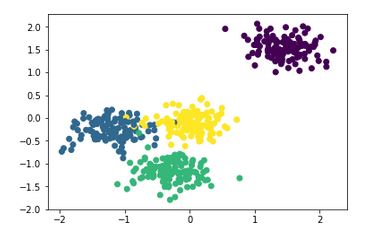
We first import the libraries and functions we might need, then use make_blobs to generate a 2-D dataset with 500 samples sorted into 4 clusters. The next step is for feature scaling, before it is fed into the DBSCAN method to make predictions. This method has been explained well at https://github.com/howardyclo/kmeans-dbscan-tutorial/blob/master/slides/clustering-tutorial-en.pdf which is also a great resource for K-means and DBSCAN.
- Python
Python
import numpy as np
import matplotlib.pyplot as plt
from sklearn import metrics

from sklearn.datasets import make_blobs

from sklearn.preprocessing import StandardScaler

from sklearn.cluster import DBSCAN
X, y = make_blobs(n_samples=500,n_features=2,

centers=4, cluster_std=1,

center_box=(-10.0, 10.0),

shuffle=True, random_state=1)
X = StandardScaler().fit_transform(X)
y_pred = DBSCAN(eps=0.3, min_samples=30).fit_predict(X)
plt.scatter(X[:,0], X[:,1], c=y_pred)
print('Number of clusters: {}'.format(len(set(y_pred[np.where(y_pred != -1)]))))
print('Homogeneity: {}'.format(metrics.homogeneity_score(y, y_pred)))
print('Completeness: {}'.format(metrics.completeness_score(y, y_pred)))
The output of that code is as follows:
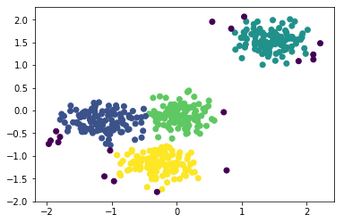
It is clear that 4 clusters are detected as expected. The black points are outliers or noise according to the DBSCAN model.
Since the dataset being analyzed has been generated by us and we know the ground truths about it, we can use metrics like the homogeneity score (checking if each cluster only has members of one class) and the completeness score (checking if all members of a class have been assigned the same cluster). The outputs for those are:
Number of clusters: 4
Homogeneity: 0.9060238108583653
Completeness: 0.8424339764592357
Which is pretty good. For unsupervised data, we can use the mean silhouette score metric instead.
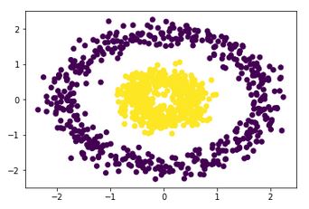
Our next example will be what really sets DBSCAN apart from K-means: a non-spherical dataset.
- Python
Python
import numpy as np
import matplotlib.pyplot as plt
from sklearn import metrics

from sklearn.datasets import make_circles

from sklearn.preprocessing import StandardScaler

from sklearn.cluster import DBSCAN
X, y = make_circles(n_samples=1000, factor=0.3, noise=0.1)

X = StandardScaler().fit_transform(X)
y_pred = DBSCAN(eps=0.3, min_samples=10).fit_predict(X)
plt.scatter(X[:,0], X[:,1], c=y_pred)
print('Number of clusters: {}'.format(len(set(y_pred[np.where(y_pred != -1)]))))
print('Homogeneity: {}'.format(metrics.homogeneity_score(y, y_pred)))
print('Completeness: {}'.format(metrics.completeness_score(y, y_pred)))
The output is:
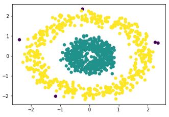
Number of clusters: 2
Homogeneity: 1.0
Completeness: 0.9611719519340282
Which is absolutely perfect. Comparatively, K-means would give a completely incorrect output like:
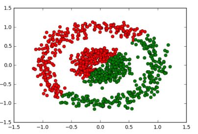
because its nature does not permit it to correctly analyze such datasets.
Applications
DBSCAN can be used for any standard application of clustering, but it is worth understanding what its advantages and disadvantages are. It is super useful when the number of clusters is not known before and must be found intuitively. It works well for arbitrarily shaped clusters as well as detecting outliers as noise. Unfortunately, since minPts and eps values are still provided explicitly, DBSCAN is not ideal for datasets with clusters of varying density since different clusters would require different values for the parameters. It also performs poorly on multidimensional data due to difficulty in estimating eps.
Now that you know the perks and pitfalls of DBSCAN, you can make an educated decision about when to use it in your analysis.
References
- https://towardsdatascience.com/the-5-clustering-algorithms-data-scientists-need-to-know-a36d136ef68
- https://sites.google.com/site/dataclusteringalgorithms/density-based-clustering-algorithm
- https://www.dummies.com/programming/big-data/data-science/how-to-create-an-unsupervised-learning-model-with-dbscan/
- https://towardsdatascience.com/how-dbscan-works-and-why-should-i-use-it-443b4a191c80
- http://scikit-learn.org/stable/auto_examples/cluster/plot_dbscan.html#sphx-glr-auto-examples-cluster-plot-dbscan-py
- https://en.wikipedia.org/wiki/DBSCAN
- https://github.com/howardyclo/kmeans-dbscan-tutorial
- https://dashee87.github.io/data science/general/Clustering-with-Scikit-with-GIFs/
- https://docs.google.com/presentation/d/1o_rTjzkK7_q672rociNBu11R5dEDlACtrWrfR34FQ3s/edit#slide=id.p