
Get this book -> Problems on Array: For Interviews and Competitive Programming
Traditional clustering algorithms perform well on convex datasets but fail to correctly recognise patterns in non-convex datasets, to overcome this issue we employ Spectral clustering. Spectral clustering is an interesting Unsupervised clustering algorithm that is capable of correctly clustering Non-convex data by the use of clever Linear algebra.
Table of contents:
- Non-Convex Data
- Data Generation
- K-Means clustering
- Spectral clustering
- Outputs & Inference
- Pros, Cons and Conclusion
Non-Convex data
In geometry, A subset of Euclidean space forms a convex set if, given any two points in the subset, the subset contains the whole line segment that joins them. Equivalently, a convex set is a subset that intersects every line into a single line segment.
To implement and visualize Spectral Clustering in python we are going to be taking the help of a few common libraries.
import numpy as np
import pandas as pd

import seaborn as sns
import matplotlib.pyplot as plt

from sklearn.cluster import KMeans
from itertools import chain
from scipy import linalg

from pandas.plotting import register_matplotlib_converters
register_matplotlib_converters()
Data Generation
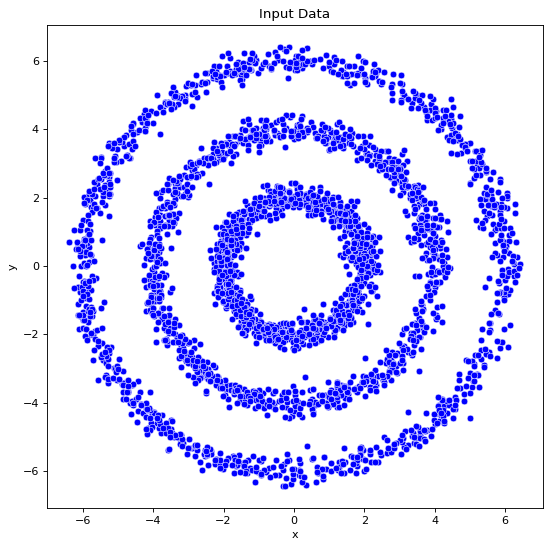
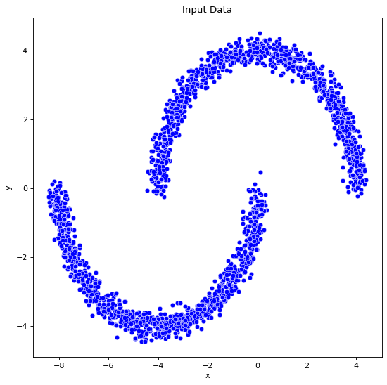
First step towards experiencing the power of spectral clustering is to aquire some non-convex data to cluster, The python function below is capable of creating 2 commonly found types of non-convex datasets (circles and crescents).
def Generate_data(r=None, noise=0.2, n=500, dset="cc"):

    x_noise = np.random.normal(loc=0, scale=noise, size=n)
    y_noise = np.random.normal(loc=0, scale=noise, size=n)

    if dset == "cc":
        r = [2, 4, 6]
        angles = np.random.uniform(low=0, high=2 * np.pi, size=n)
        # create Concentric Circle Dataset
        x = chain(*[i * np.cos(angles) + x_noise for i in (r)])
        y = chain(*[i * np.sin(angles) + y_noise for i in (r)])

    else:
        # Create Moon Dataset
        r = 4
        angles1 = np.random.uniform(low=0, high=np.pi, size=n)
        angles = np.random.uniform(low=0, high=np.pi, size=n)
        x1 = [r * np.cos(angles) + x_noise]
        y1 = [r * np.sin(angles) + y_noise]

        x2 = [-r + 4 * np.cos(angles1) + x_noise]
        y2 = [-r * np.sin(angles1) + y_noise]

        x = chain(*x1, *x2)
        y = chain(*y1, *y2)

    return pd.DataFrame(data={"x": x, "y": y})
The function Generate_data takes 4 input parameters,
r- list specifying the radius of the circles to be generatednoise- specifying the standard distribution of the noise being added to the data points.n- specifying the number of data points to be created.dset- specifying the type of dataset to create (circle/crescent)
and returns a dataframe of 2 columns with x and y coordinates of each data point created.
Using this we can create and visualize the datasets using the following sections of code,
data_df=Generate_data(noise=0.2,n=1000,dset="cc")
fig, ax = plt.subplots()
sns.scatterplot(x="x", y="y", color="blue", data=data_df, ax=ax)
ax.set(title="Input Data")
data_df=Generate_data(noise=0.2,n=1000,dset="moon")
fig, ax = plt.subplots()
sns.scatterplot(x="x", y="y", color="blue", data=data_df, ax=ax)
ax.set(title="Input Data")
K-Means Clustering
For the sake of comparsion with traditional clustering algortihms we will first be implementing commomly used clustering algorithm K-means on the created data.
The steps to implement K-means Clustering is,
- Select the number K to decide the number of clusters.
- Select random K points or centroids. (It can be other from the input dataset).
- Assign each data point to their closest centroid, which will form the predefined K clusters.
- Calculate the variance and place a new centroid of each cluster.
- Repeat the third steps, which means reassign each datapoint to the new closest centroid of each cluster.
- If any reassignment occurs, then go to step-4 else go to FINISH.
- The model is ready
The required mathematical components of K-Means clustering are,
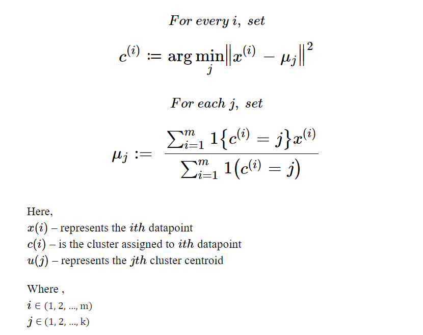
these formulas can be understood as,
- The first formula assigns the cluster to a datapoint
iby computing the cluster centre from which the distance is minimum but it returns "arg-min(j)" which identifies the cluster not the distance value. - The second formula recomputes the cluster centre after every iteration of assigning clusters to all datapoints, for a given j the recalculated cluster centre can be found by the mean of data points of the cluster.
To implemet k-means we need require a fair value of k which can obtained by performing the WCSS(Within Cluster Sum of Square)/elbow method with the code below,
WCSS_array=np.array([])
for K in range(1,5):                      # running it for k = 1-> 5
    kmeans=KMeans(X,K)                    # Collecting the Data points
    kmeans.fit(n_iter)
    Output,Centroids=kmeans.predict()     # Collecting the centroids
    wcss=0

    for k in range(K):                    # Comparing for each k value
        # sum of squared distances of sample to their closest cluster center
        wcss+=np.sum((Output[k+1]-Centroids[k,:])**2)
    WCSS_array=np.append(WCSS_array,wcss)
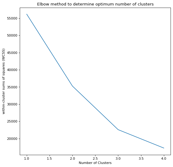
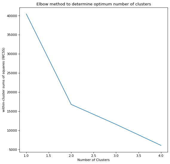
We can see that the Elbow plot bends sharply at k=3 and k=2 for each of the datasets respectively. With this value we will implement the K-means algorithm like so,
class KMeans:
    def __init__(self,X,K):
        # constructor of class KMeans which initilizes X and K variables
        self.X=X
        self.Output={}
        self.Centroids=np.array([]).reshape(self.X.shape[1],0)
        self.K=K
        self.m=self.X.shape[0]

    def kmeanspp(self,X,K):
        i=rd.randint(0,X.shape[0])
        Centroid_temp=np.array([X[i]])
        for k in range(1,K):
            D=np.array([])
            for x in X:
                D=np.append(D,np.min(np.sum((x-Centroid_temp)**2)))
            prob=D/np.sum(D)
            cummulative_prob=np.cumsum(prob)
            r=rd.random()
            i=0
            for j,p in enumerate(cummulative_prob):
                if r<p:
                    i=j
                    break
            Centroid_temp=np.append(Centroid_temp,[X[i]],axis=0)
        return Centroid_temp.T

    def fit(self,n_iter):
        #randomly Initialize the centroids
        self.Centroids=self.kmeanspp(self.X,self.K)

        """for i in range(self.K):
            rand=rd.randint(0,self.m-1)
            self.Centroids=np.c_[self.Centroids,self.X[rand]]"""

        #compute euclidian distances and assign clusters
        for n in range(n_iter):
            EuclidianDistance=np.array([]).reshape(self.m,0)
            for k in range(self.K):
                tempDist=np.sum((self.X-self.Centroids[:,k])**2,axis=1)
                EuclidianDistance=np.c_[EuclidianDistance,tempDist]
            C=np.argmin(EuclidianDistance,axis=1)+1
            #adjust the centroids
            Y={}
            for k in range(self.K):
                Y[k+1]=np.array([]).reshape(2,0)
            for i in range(self.m):
                Y[C[i]]=np.c_[Y[C[i]],self.X[i]]

            for k in range(self.K):
                Y[k+1]=Y[k+1].T
            for k in range(self.K):
                self.Centroids[:,k]=np.mean(Y[k+1],axis=0)

            self.Output=Y


    def predict(self):
        # With Centroids
        return self.Output,self.Centroids.T
        # Without Centroids
        # return self.Output

    def WCSS(self):
        wcss=0
        for k in range(self.K):
            wcss+=np.sum((self.Output[k+1]-self.Centroids[:,k])**2)
        return wcss
Spectral Clustering
The steps involved in implementing the Spectral Clustering are,
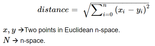
- Form a distance matrix
- Transform the distance matrix into an affinity matrix A
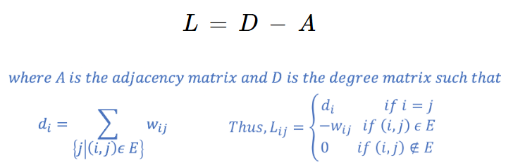
- Compute the degree matrix D and the Laplacian matrix L = D – A.
- Find the eigenvalues and eigenvectors of L.
- With the eigenvectors of k Smallest eigenvalues computed from the previous step form a matrix U.
- Normalize the vectors.
- Cluster the data points in k-dimensional space
It is important to note that although Spectral Clustering is understood as clustering algorithm its really more of a perspective changing technique employed on the input data to help the clustering part of the Spectral Clustering algorithm easily and concretely distinguish the data into clusters better.
Mathematical components of Spectral clustering are,
Elements of the weighted Adjacency matrix A is popluated by,
Our goal then is to transform the space so that when the 2 points are close, they are always in same cluster, and when they are far apart, they are in different clusters. We need to project our observations into a low-dimensional space. For this, we compute the Graph Laplacian, which is just another matrix representation of a graph and can be useful in finding interesting properties of a graph. The Laplacian (L) can be formed by,
The purpose of computing the Graph Laplacian L was to find eigenvalues and eigenvectors for it, to project and transform the data points into a low-dimensional space (spectral domain). This can be done by solving,
l*lambda = lambda*v
In Essence,
We need a mathematical representation of the all-data points to cluster them, to get this representation we form the Graph Laplacian.
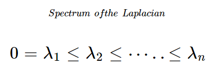
- The Eigen Values of the Graph Laplacian has a few interesting advantageous properties,
- The number of 0 Eigen values represent the number of completely disconnected portions of graphs
- The value of any Eigen value represents the level of connectivity of the portion of the graph
Now we have considered k lowest Eigen valued, Eigen vectors, so within the dimension of the considered vectors the portions of graphs are least connected. In other words, the clusters are distinct because the data points become more distinguishable in lower dimension while using distance metric.
The Dimensionality changes with each step when we consider n data points are,
- The dimension of
L,D&Awill benxn - The number of Eigen values and Eigen vectors of
Leach aren. Each Eigen vector is of dimensionnx1 - Now considering
klowest Eigen valued, Eigen vectors and forming a matrixUof dimensionnxk
Finally, we cluster the data using U.
Each of the steps in python can be implemented using the corresponding functions,
def generate_graph_laplacian(df):
    input=np.array(df)
    # calculate the distance matrix
    A = np.zeros((df.shape[0],df.shape[0]))
    for i in range(A.shape[0]):
        A[i,:]=np.sqrt(np.sum((input-input[i,:])**2,axis=1))
    # threshold the distance matrix
    A[A>0.5]=0
    # calculate the graph laplacian
    D=np.diag(np.sum(A,axis=1))
    L = D-A
    return L

def compute_spectrum_graph_laplacian(graph_laplacian):
    """Compute eigenvalues and eigenvectors and project
    them onto the real numbers.
    """
    eigenvals, eigenvcts = linalg.eig(graph_laplacian)
    eigenvals = np.real(eigenvals)
    eigenvcts = np.real(eigenvcts)
    return eigenvals, eigenvcts

def project_and_transpose(eigenvals, eigenvcts, num_ev):
    """Select the eigenvectors corresponding to the first
    (sorted) num_ev eigenvalues as columns in a data frame.
    """
    eigenvals_sorted_indices = np.argsort(eigenvals)
    indices = eigenvals_sorted_indices[:num_ev]

    proj_df = pd.DataFrame(eigenvcts[:, indices.squeeze()])
    proj_df.columns = [f"v_{str(c)}" for c in proj_df.columns]
    return proj_df

def run_k_means(df, n_clusters):
    """K-means clustering."""
    k_means = KMeans(random_state=25, n_clusters=n_clusters)
    k_means.fit(df)
    return k_means.predict(df)

def spectral_clustering(df, n_clusters):
    """Spectral Clustering Algorithm."""
    graph_laplacian = generate_graph_laplacian(df)
    eigenvals, eigenvcts = compute_spectrum_graph_laplacian(graph_laplacian)
    proj_df = project_and_transpose(eigenvals, eigenvcts, n_clusters)
    cluster = run_k_means(proj_df, proj_df.columns.size)
    return [f"c_{str(c)}" for c in cluster]
Outputs & Inference
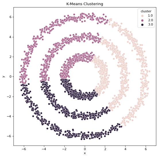
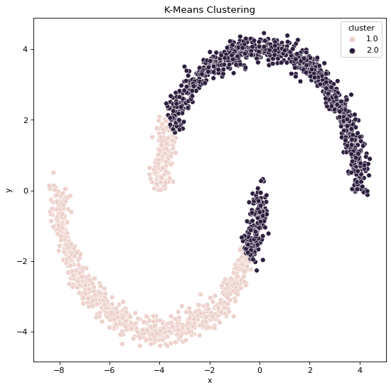
Using K-Means Clustering,
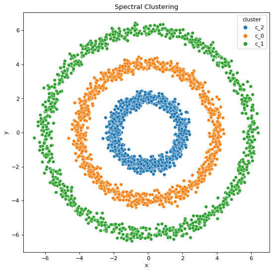
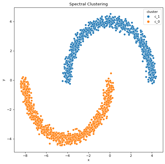
Using Spectral Clustering,
We can infer,
From repeatedly applying conventional K-Means Clustering on Convex datasets we know that the generally we don’t face any problems when it comes to clustering performance with respect to True Dataset patterns.
But, when we apply K-Means Clustering on Non-Convex datasets we can intuitively see that the output is being guided by simple distance measure Clustering formula, this does not sufficiently equip the algorithm to identify clearly visible patterns present within the Data.
To overcome this drawback, we assist the algorithm by reducing the dimensionality by representing the data in a low dimension space (spectrum), this is done easily via the use of the mathematics discuss earlier, simply put we just help the algorithm ignore some of the less relevant information which makes the global pattern recognition effective.
All these statements are validated by the clustering outputs obtained where we can see the resulting cluster patterns and data generation patterns are not the same when it comes to the output clusters formed by K-Means algorithm whereas they are the same when it comes to the output clusters formed by Spectral Classification algorithm.
Pros, Cons and Conclusion
Advantages of Spectral Clustering are,
- Makes no major assumptions about the cluster statistics.
- K-Means clustering approaches The points given to a cluster are assumed to be spherical around the cluster centre when clustering. This is a big assumption to make, and it may or may not be true. In such instances, spectral clustering aids in the formation of more precise clusters.
- It's simple to use and produces good clustering results. It can appropriately cluster observations that belong to the same cluster but are separated by dimension reduction from observations in other clusters.
- Fast enough for sparse data sets with thousands of elements.
On the other hand, Disadvantages of Spectral Clustering are,
- The final phase of K-Means clustering indicates that the clusters are not always the same. They may differ based on the initial centroids chosen.
- Large datasets are computationally expensive.
- This is because eigenvalues and eigenvectors must be determined before clustering can be performed on these vectors. This may significantly increase the temporal complexity of large, dense collections.
In hindsight, we use spectral clustering when we find that convential simple clustering aglorithms fail to identify data patterns as expected.
With this article at OpenGenus, you must have the complete idea of Spectral clustering.