K-means Clustering

If you are unfamiliar with the clustering problem, it is advisable to read the Introduction to Clustering available at OpenGenus IQ before this article.

K-means clustering is a prime example of unsupervised learning and partitional clustering. It works on an unlabeled dataset to divide it into a number of sections, such that the points in each section are more similar to each other across all features than they are to points in other clusters. It is one of the most popular machine learning algorithms and finds widespread application across several fields.

K-means clustering is also loosely connected to the popular classifier called K Nearest Neighbors due to some similarities in constituent operations, but it is worth remembering that classification (for which KNN is used) is a subset of supervised learning and is entirely separate from clustering.

Algorithm and Examples

We now move to the methodology behind k-means and the actual algorithm, which is as follows:

1. Initialize k "means" or clusters in the given data space of d dimensions
2. Randomly assign each point to one of the cluster centres.
3. Compute the centroids for each cluster using something akin to the midpoint/centroid theorem which averages out the coordinates of all the points.
4. In the next iteration, assign each data point to the cluster centre closest to it (minimum distance as computed via Euclidean, Chebyshev, or Manhattan methods)
5. Recompute the cluster centres.
6. Repeat steps 4 and 5 until an optimal solution is found. This is typically considered to be when two iterations return the same clustering.

As we can understand here, each iteration gives us the local optimum clustering, and the process is stopped when we reach an apparent global optimum. We say apparent here because due to randomness in the initial point assignment to clusters, our algorithm may well return different clustering when run repeatedly.

Demonstration

Example 1

Our elementary data set has only 4 points:

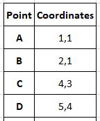
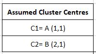
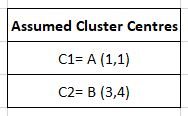
We have decided that the desired number of clusters or k will be 2. Here we initialize the cluster centres as the first 2 points (you are free to initialize them as any points, not only from the dataset but anywhere in the vector space)

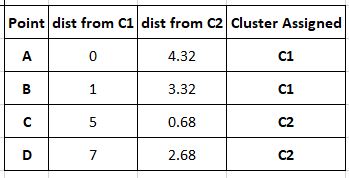
The next step is the first iteration of the process, where we find distances of each point from our cluster centres and assign a cluster to the point based on the centre closest to it. Here our distance measure is assumed to be Manhattan distance (covered in the article on clustering. d= |x2-x1| + |y2-y1|) for the sake of simplicity.

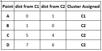
Our new clusters are C1= (A) and C2= (B,C,D) Now that our clusters are populated, we must update the cluster centre to ensure it actually corresponds to the centre of the new cluster. This is done by averaging out the coordinates using the formula:

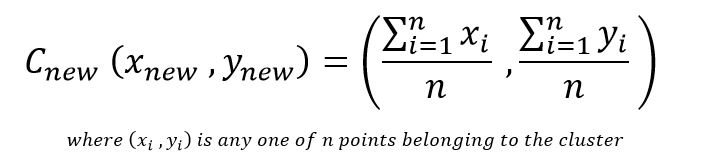
C1 remains (1,1) and C2 is now (2+4+5)/3 , (1+3+4)/3 or (3.66, 2.66)

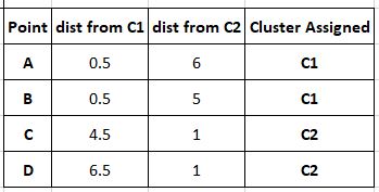
We now move to the next iteration of the loop and repeat what we did in the first.

Since point B is now closer to C1 than to C2, it is considered to be a part of C1.
Our clusters are C1 (A,B) and C2 (C,D). We must update our cluster centres.

C1 becomes (1+2)/2 , (1+1)/2 or (1.5, 1) and C2 becomes (4+5)/2, (3+4)/2 or (4.5, 3.5)

Moving to the next iteration

We clearly see that no points are relocated to new clusters, meaning no updation of cluster centres will take place and the next iteration would be pointless, aka we have reached an optima. We terminate the clustering process with the resultant clusters as C1 (A,B) and C2 (C,D).

Example 2

Let's assume we have a small data set of 6 points:

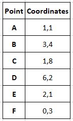
We have decided that the desired number of clusters or k will be 2. Here we initialize the cluster centres as the first 2 points.

The clusters are assigned based on Manhattan distance as above.

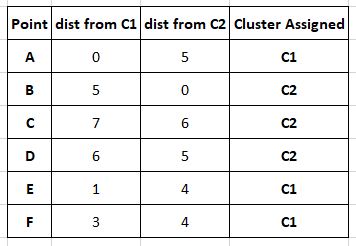
The centroids are recomputed.

The new cluster centres are
C1= (1+2+0)/3 , (1+1+3)/3 or (1,1.66)
C2= (3+1+6)/3 , (4+8+2)/3 or (3.33,4.66)

We now move to the next iteration of the loop and repeat what we did in the first.

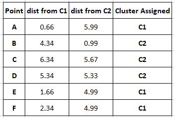
It is evident from here that the second iteration does not cause a change in the clustering and our cluster centres have not changed, thus making it pointless to push to the next iteration. The clustering process is deemed complete and our clusters are: (A,E,F) and (B,C,D).

Complexity

• Best Case: If the desired number of clusters is 1 or n, the clustering algorithm has O(n) complexity.
• Worst Case:
  • In a general space with d dimensions for just 2 clusters, clustering is NP-hard.
  • For any number of clusters k, clustering is an NP-hard problem.
• Average Case: For a fixed number of dimensions d and clusters k: O(n^(dk+1)) complexity.

Implementations

To visualize K-means clustering we use tools provided already in R, a specialized language for mathematicians, scientists, and statisticians. We perform clustering on the Iris dataset, which you can read about here: https://archive.ics.uci.edu/ml/datasets/iris

• R

library(datasets)
data("iris")
x=iris[,3:4]
model=kmeans(x,3)
library(cluster)
clusplot(x,model$cluster,color=T,shade = T,lines=0,main = 'Clusters',xlab = 'Petal

Length' , ylab = 'Petal Width',sub='')

We first load the dataset and choose our features/dimensions to be petal length and width. Next, we train a kmeans model to find 3 distinct clusters that we know exist here. Finally we plot this clustering with some modifiers regarding the coloring, shading and axis labels. This returns the output: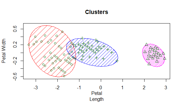

A similar implementation can be performed on Python as shown by http://constantgeeks.com/playing-with-iris-data-kmeans-clustering-in-python/

• Python2.7

from sklearn import datasets
from sklearn.cluster import KMeans
import pandas as pd
import numpy as np
import matplotlib.pyplot as plt
iris = datasets.load_iris()
x = pd.DataFrame(iris.data, columns=['Sepal Length', 'Sepal Width', 'Petal Length', 'Petal Width'])

y = pd.DataFrame(iris.target, columns=['Target'])
plt.figure(figsize=(12,3))
colors = np.array(['red', 'green', 'blue'])
model = KMeans(n_clusters=3)

model.fit(x)
plt.figure(figsize=(12,3))
colors = np.array(['red', 'green', 'blue'])
predictedY = np.choose(model.labels_, [1, 0, 2]).astype(np.int64)
plt.subplot(1, 2, 1)

plt.scatter(x['Petal Length'], x['Petal Width'], c=colormap[y['Target']], s=40)

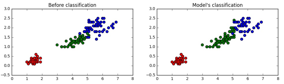
plt.title('Before classification')
plt.subplot(1, 2, 2)

plt.scatter(x['Petal Length'], x['Petal Width'], c=colormap[predictedY], s=40)
plt.title("Model's classification")

The functions performed here are essentially similar, and we plot the datapoints based on the labels given on the left and then the output of the clustering algorithm on the unlabeled data on the right to compare the same.

Those interested in an implementation of the algorithm from scratch without any libraries can visit https://github.com/stuntgoat/kmeans/blob/master/kmeans.py as well as https://github.com/MrDupin/Machine-Learning/blob/master/Clustering/kMeans - Standard/kMeans.py

Applications

You must already have come across some broad examples of how clustering is used in the article about clustering. Some interesting, albeit more specific examples are:

• Document and Web Page Classification: Aggregators like Google Search and Google News must find all pages that correspond to a particular keyword, query, or topic and display them together for user convenience
• Customer Segmentation: Employed by almost all companies to better understand the habits and needs of your customers and target audience so that you may serve them better or provide more targeted advertisements.
• CDR Analysis: Employed by all major telecom providers, call records of customers are analyzed to single out groups of customers to whom tailor-made plans can be delivered to serve them best.
• Criminal Profiling: Law enforcement agencies collect, organize, and analyze criminal data to find possible links or associations.
• Fraud Detection: Credit card companies and insurance companies employ clustering to detect fraudulent transactions or claims by employing a technique called outlier analysis to detect individual elements that feel abnormal due to drastic differences from past trends.

It is also worth noting that there are some differences between hierarchical and K-means clustering:

• K-means clustering generally performs better with big data than hierarchical due to hierarchical having a quadratic time complexity.
• Hierarchical clustering can reproduce the same clustering if performed twice on the same data, but K-means tends to produce different outputs on multiple execution due to innate randomness in cluster assignment during the first iteration.
• For hierarchical clustering, we are able to stop at whatever number of clusters seems appropriate from the dendrogram or the output, but we go into K-means knowing what the desired number of clusters (k) is. Another valid approach is to iterate k values from 1 to n and stop execution when a desired clustering seems visible. This is however not computationally efficient.

References

• https://en.wikipedia.org/wiki/K-means_clustering
• http://aris.me/contents/teaching/data-mining-2016/slides/partitional-clustering.pdf
• https://www.datascience.com/blog/k-means-clustering
• https://github.com/stuntgoat/kmeans/blob/master/kmeans.py
• https://github.com/MrDupin/Machine-Learning/blob/master/Clustering/kMeans - Standard/
• http://constantgeeks.com/playing-with-iris-data-kmeans-clustering-in-python/
• https://archive.ics.uci.edu/ml/datasets/iris